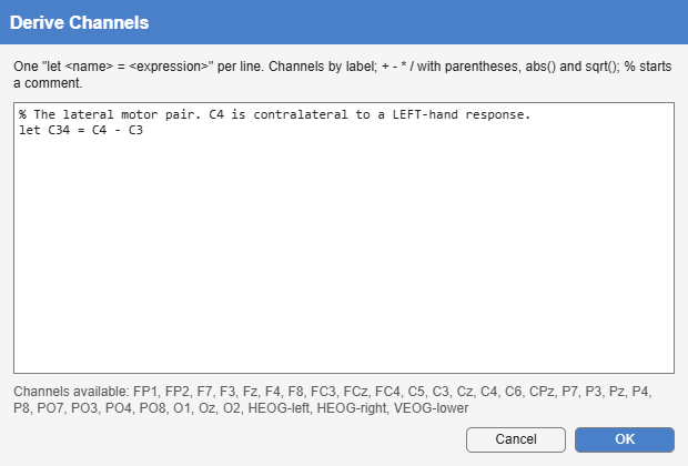
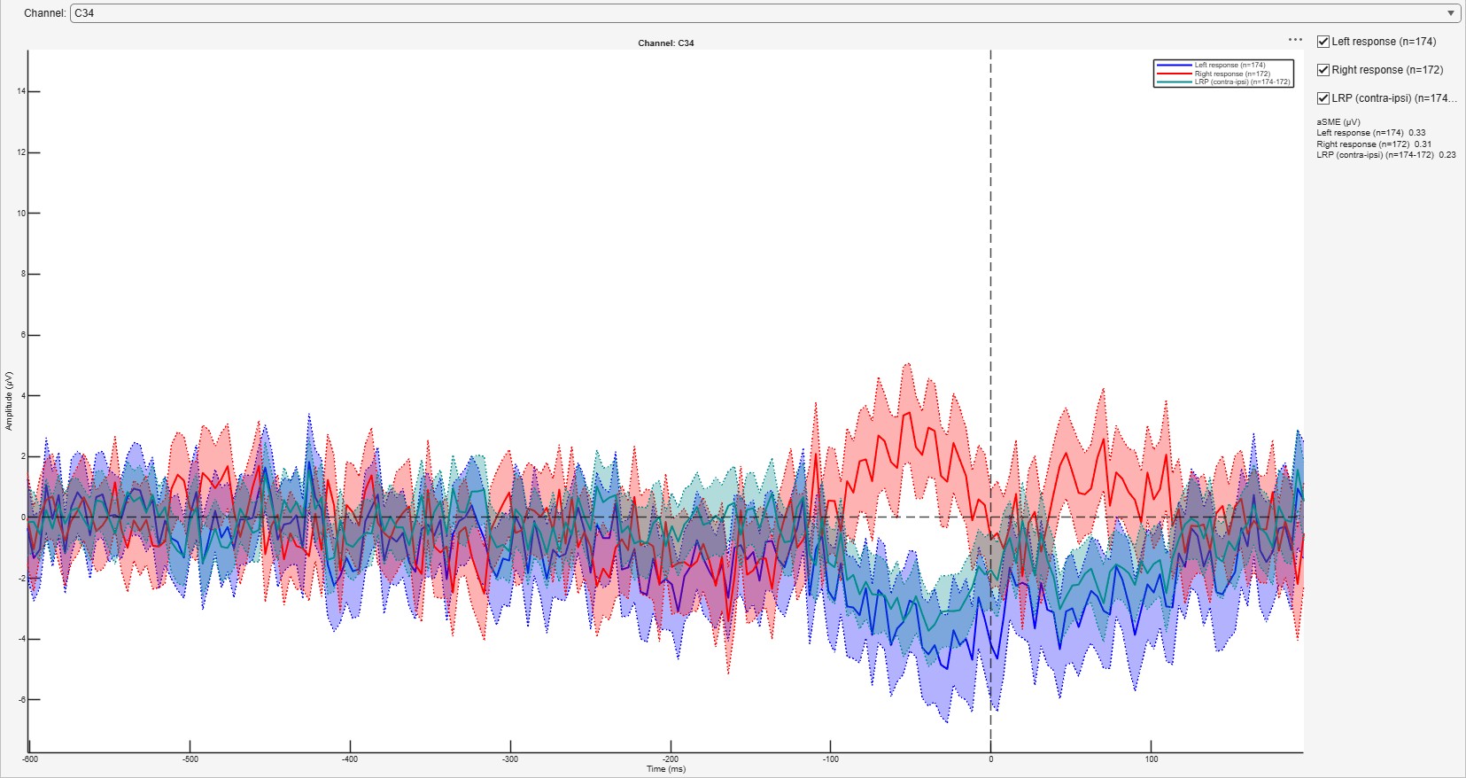
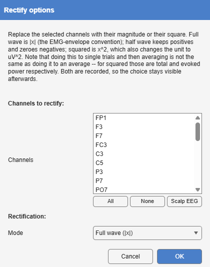
Alakazam is an interactive MATLAB workbench for the analysis of EEG and event-related potentials (ERPs). It loads a recording, lets the researcher apply a sequence of processing steps to it, and keeps the whole processing history as an explorable tree rather than as the one-off result of a script. Every step can be inspected, revised, replayed on other recordings, and written out as code.
It is built on EEGLAB’s EEG data structure (Delorme and Makeig 2004), so every intermediate result can be handed to EEGLAB, ERPLAB (Lopez-Calderon and Luck 2014) or FieldTrip (Oostenveld et al. 2011) unchanged, and its methods follow established practice for ERP research as described by Luck (2014a), in Luck’s open textbook (Luck 2022), in the protocol of Pütz et al. (2025), which walks through the same workflow from designing an ERP task and recording it to preprocessing and exporting the measures for statistical analysis, and in the field’s publication guidelines (Keil et al. 2014; Pernet et al. 2020).
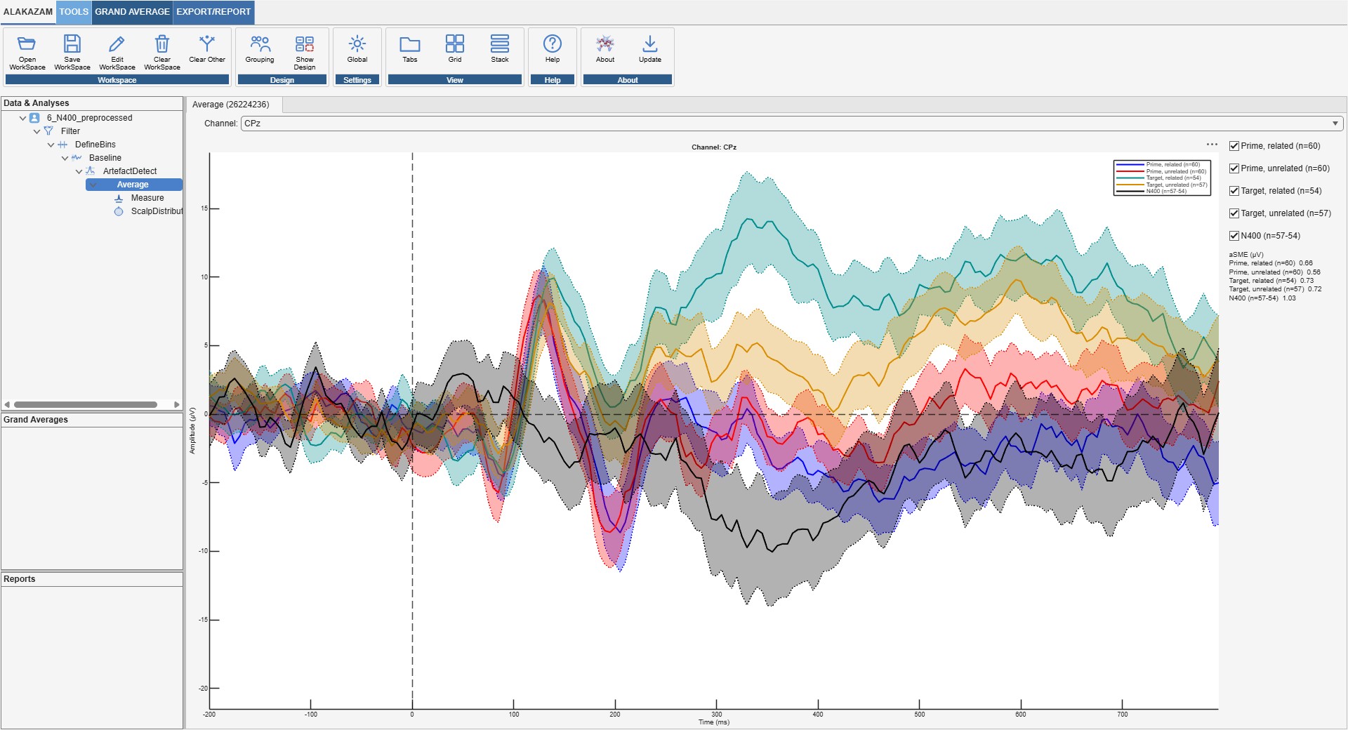
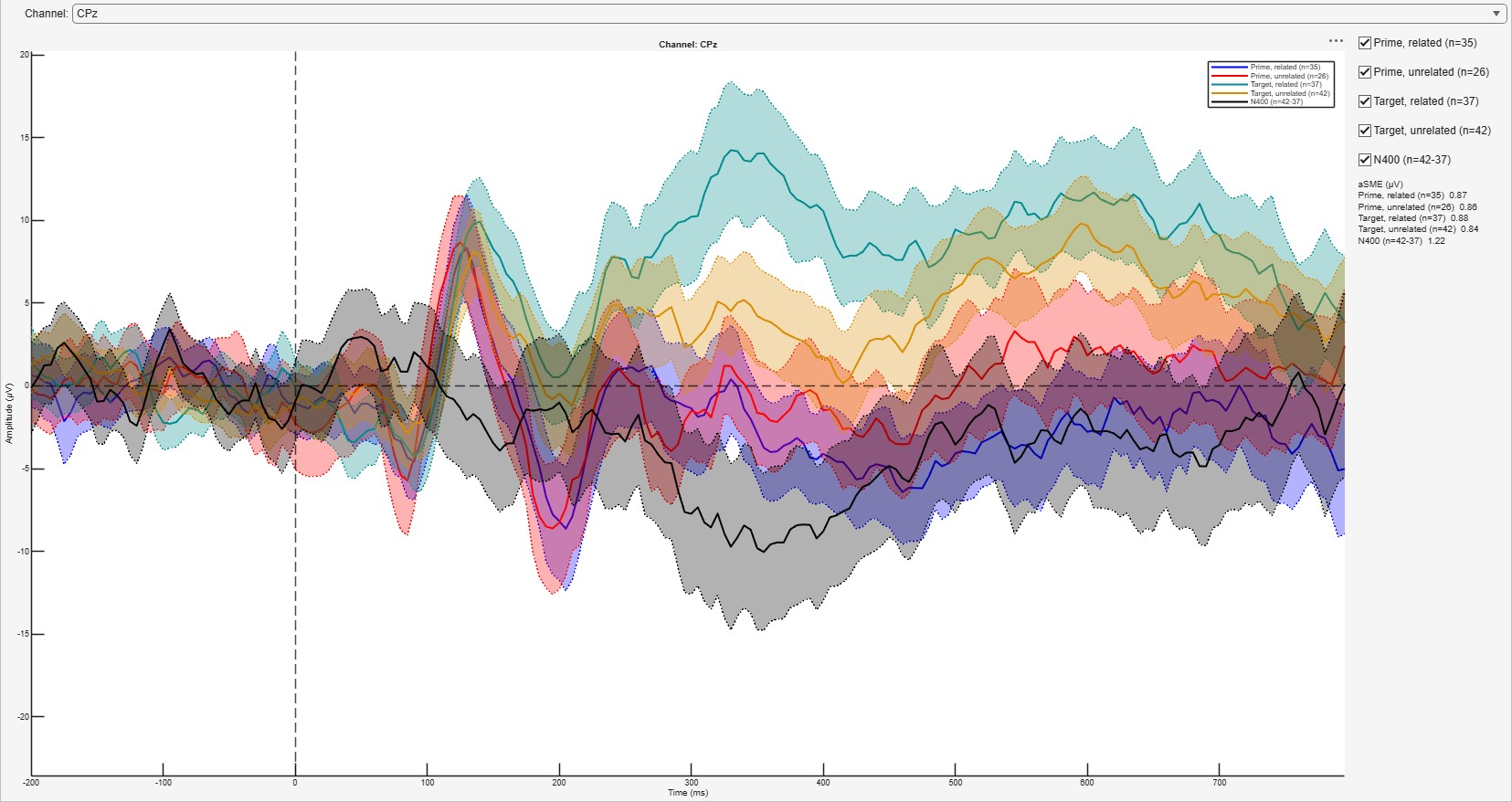
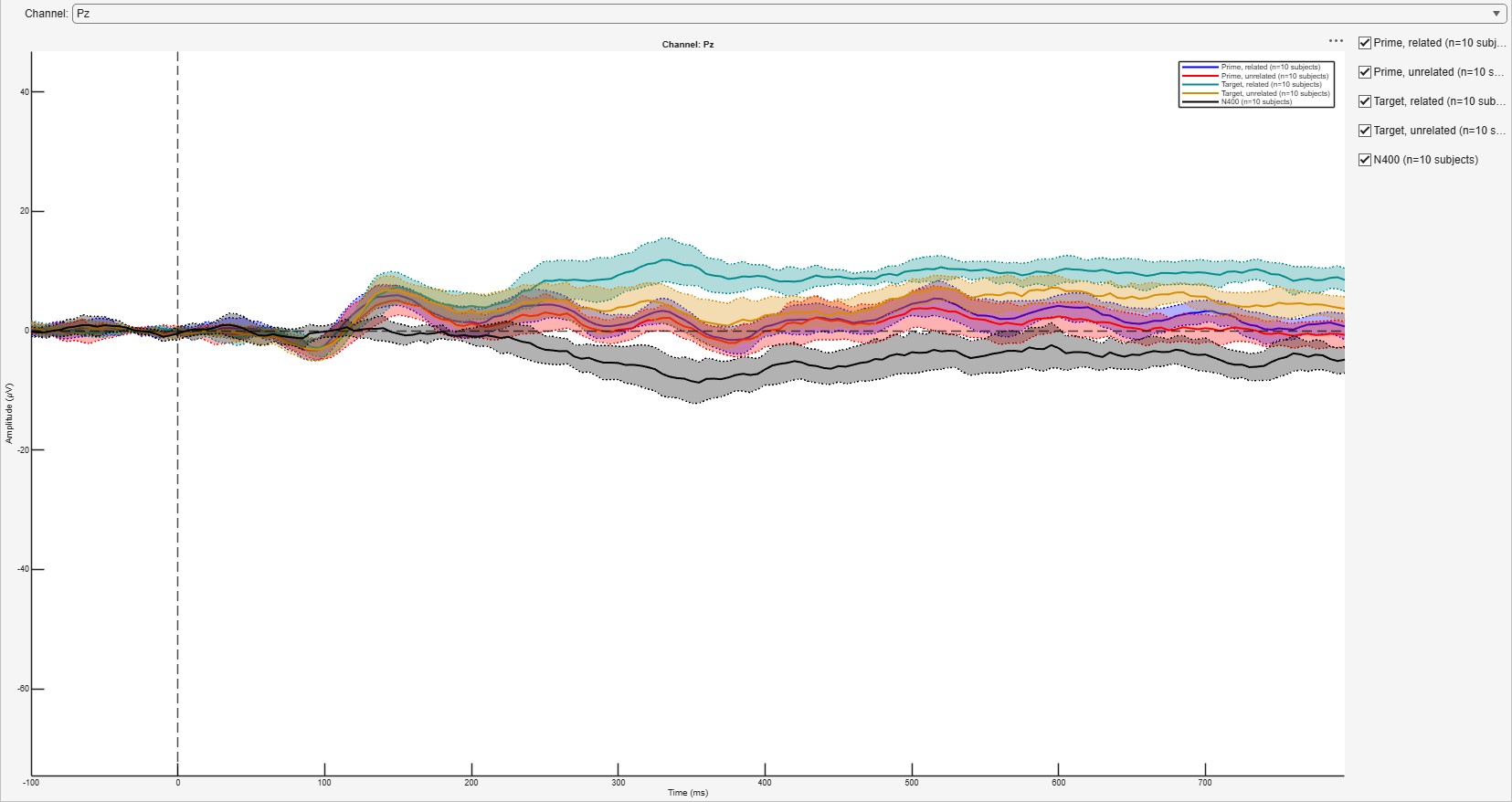
Figure 1.1: The main window: the ribbon along the top, the three trees on the left (here one recording and the branch the N400 template built from it) and the selected Average node’s waveforms at CPz on the right.
1.1 What it does
The analyses Alakazam supports, and where this manual describes each:
The ERP pipeline: filtering, re-referencing, artefact correction and rejection, epoching by a small language for describing conditions, baseline correction, averaging, and measurement of amplitudes, areas and latencies (Chapter 7 to Chapter 11).
Statistics: design-aware reports that choose the test the design calls for, from paired t-tests to linear mixed models with Bayes factors (Chapter 13), and cluster-based permutation tests over the scalp or the cortical surface (Chapter 14).
Data quality: per-subject and per-condition trial loss, noise, the standardised measurement error and the dependability of each score (Chapter 15).
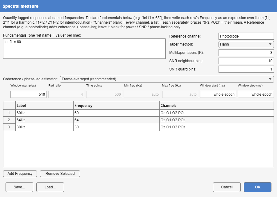
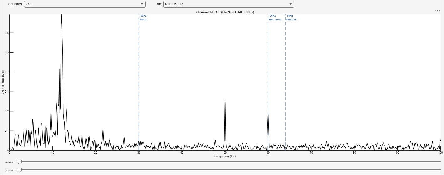
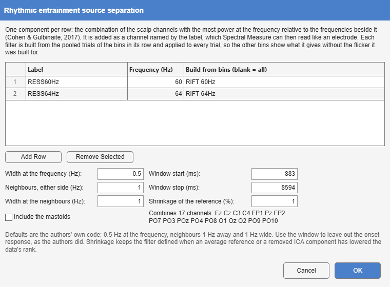
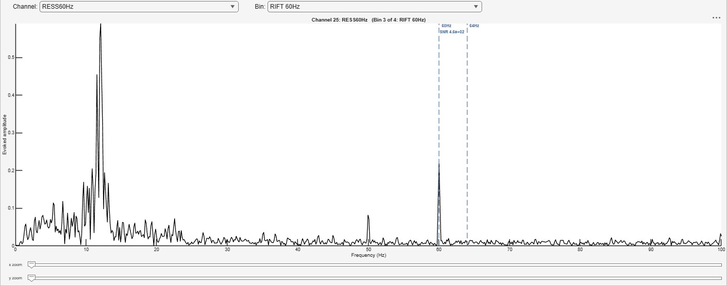
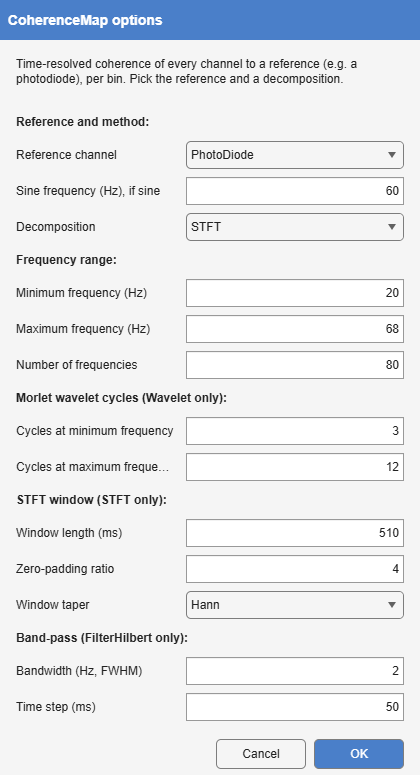
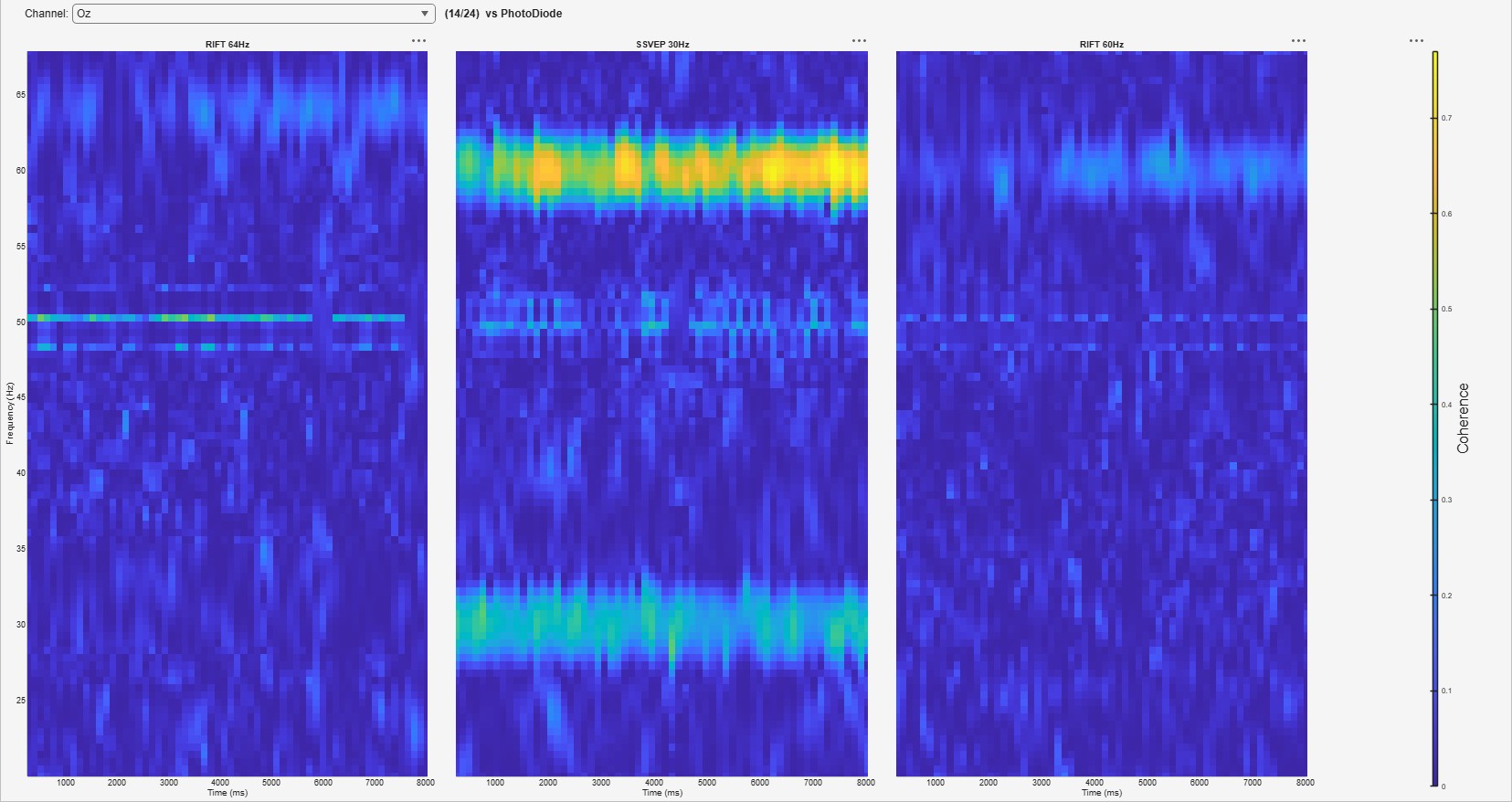
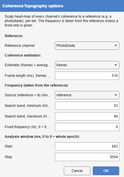
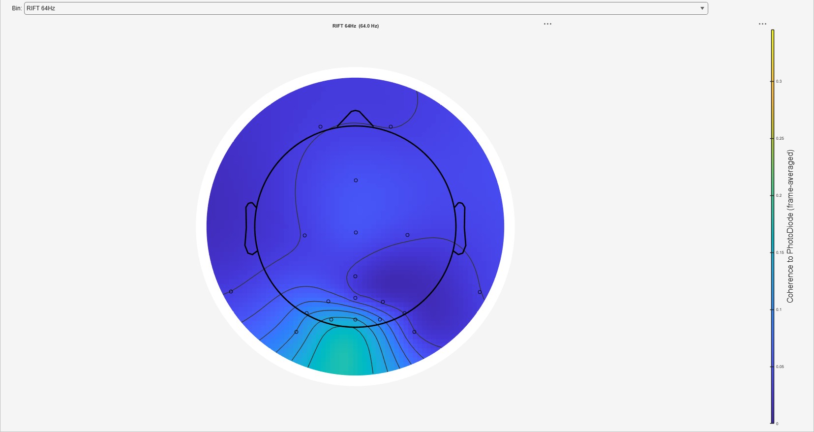
Frequency tagging and steady-state responses: power, signal-to-noise ratio, phase-locking and coherence to a photodiode, time-resolved coherence maps and spatial filters (Chapter 16).
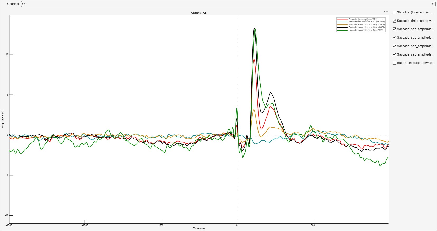
Overlapping responses: regression-based deconvolution for designs in which one event’s response overlaps the next, such as free viewing, reading or fast presentation (Chapter 17), and co-registration with an eye tracker.
Source estimation on a template cortex, with the limits of what such an estimate can show stated alongside it (Chapter 18).
Reproducibility: templates that replay a pipeline on new recordings, and export of the whole analysis as a runnable MATLAB script (Chapter 19).
1.2 Principles
A few decisions run through the whole application, and knowing them makes its behaviour predictable.
The raw data is never modified. Each recording is a root in the tree. Every processing step produces a new node beneath the node it was applied to, and its result is written to a cache folder, never to the folder that holds the recordings.
Every result knows how it was made. A node records the transformation that produced it and the exact options it used. That record is what lets a step be revised (Recalculate), replayed on another recording (drag and drop, Apply to All Raw Files), saved as a template, and written out as code. Steps that change what the numbers mean without changing how they look, such as interpolating a channel or removing ICA components, also record what they did, so that the data-quality report can show it.
The tree branches. A second preprocessing choice does not replace the first; it becomes a second branch from the same node, and the two results can be compared side by side. Robustness to a preprocessing choice is something to be checked rather than assumed (Luck and Gaspelin 2017).
Numbers are shown with the signal they came from. The statistical reports draw the waveforms and spectra behind every measurement, with the measurement window marked, so that a window over the wrong peak or a component that is not there cannot hide behind a well-formed test.
Library calls where they are faithful. Where EEGLAB, FieldTrip or another established toolbox implements a method, Alakazam calls it rather than reimplementing it, and says so; where it implements a method itself, the method and its validation are described (see the provenance notes in each transformation’s section).
1.3 Who this manual is for
The manual assumes a reader who knows what an ERP is, what a filter does to one and why trials are averaged, and who wants to know precisely what each step in Alakazam computes, with which defaults, and on what methodological grounds. It does not assume any familiarity with MATLAB programming; the chapter on reproducibility is the only one that shows code.
Conventions used throughout:
Interface elements are in bold: a ribbon tab, a button, a field.
A path such as Tools > 1. Preprocessing > Filter names a ribbon tab, a group on it, and a button in the group.
Transformations are named by their ribbon label; where the internal name differs (the one a template or an exported script uses), both are given once, in the transformation’s own section.
Times are in milliseconds relative to the time-locking event, and voltages in microvolts, unless stated otherwise.
1.4 The data in this manual
Every figure in this manual was made by Alakazam itself from openly available recordings, regenerated by a script that drives the application (see the developer guide). The datasets are:
ERP CORE(Kappenman et al. 2021): the N400, LRP, N2pc and MMN experiments, as distributed with Luck’s textbook (Luck 2022).
Rapid invisible frequency tagging (RIFT) recordings with a photodiode (Dimigen et al. 2025).
Ehinger and Dimigen’s face data: one participant of a face discrimination task with involuntary saccades and button presses (Ehinger and Dimigen 2019).
EYE-EEG’s reading data: natural sentence reading with a co-registered eye tracker (Dimigen et al. 2011).
The recordings are not part of the Alakazam repository; DATA.md there says where to obtain each.
1.5 Citing Alakazam and the methods it runs
When a publication reports an analysis made with Alakazam, cite the software and, more importantly, the methods the analysis used: EEGLAB (Delorme and Makeig 2004) for the data structure and the preprocessing functions it wraps, and the specific methods named in each transformation’s section of this manual (for instance ICLabel (Pion-Tonachini et al. 2019) for automatic component classification, the Unfold toolbox (Ehinger and Dimigen 2019) for deconvolution, or FieldTrip (Oostenveld et al. 2011) for cluster statistics and source estimates). Export as Code (Section 19.4) writes the complete pipeline with the options actually used, which is the most precise methods description available.
2 Installation
2.1 Requirements
Alakazam runs in MATLAB on Windows, macOS and Linux. It needs:
MATLAB with uifigure support (the interface is built entirely on that component family), a recent release;
the Signal Processing Toolbox, used by the filters and the taper windows of the spectral transformations;
the Statistics and Machine Learning Toolbox, used by EEGLAB and some of its plugins;
EEGLAB(Delorme and Makeig 2004), which Alakazam initialises for itself when it is not already on the path, leaving the saved MATLAB path unchanged.
The Parallel Computing Toolbox is advised but not required. Three things use it, and each runs serially without it, only more slowly: Apply to All Raw Files processes several recordings at once (on nine RIFT recordings, 215 s on three workers against 364 s one at a time); cluster statistics split their permutations across workers; and GEDAI uses a GPU when one is present. The workers are local processes, so no cluster or MATLAB Parallel Server is involved.
For the statistical reports, Quarto and R are needed (see Chapter 13). Quarto is bundled with RStudio; the R packages a report uses are installed by the report itself the first time it renders. Without them the report’s source and its data are still written, and can be rendered later.
2.2 Toolboxes installed on first use
Several methods rely on toolboxes that are not bundled with Alakazam. Each is downloaded the first time a transformation needs it, after a dialog that names the toolbox, its licence and its size and asks for consent. Most are pinned to a specific version, so that a result can be reproduced on another machine later. GEDAI is the exception: AutoGEDAI keeps it at its newest release, and records the release that ran with each result (Section 8.6).
Table 2.1: Toolboxes Alakazam installs when first needed.
GEDAI’s licence allows personal and noncommercial research use only; commercial use needs a separate licence from its authors.
2.3 Getting Alakazam
Either clone the repository or download a packaged release from the releases page. A release is the same source tree with this manual already built for the Help button; a clone builds it on the first press of Help, which needs Quarto.
2.4 Starting it
From the repository root, in MATLAB:
startAlakazam
startAlakazam adds Alakazam’s source folder to the path and opens the application, which then adds the toolkits it needs. At startup it checks for the Signal Processing and Statistics toolboxes and warns, without stopping, if either is missing.
To start with a particular workspace rather than the default one, name it:
startAlakazam('MyStudy.wksp')
2.5 Updating
The Update button on the Alakazam tab checks for a newer release. When there is one it downloads it, and the new version takes over the next time startAlakazam runs. A git clone is not updated this way; use git.
3 Getting started
This chapter is a guided first session. By the end of it you will have loaded a recording, filtered it, cut it into epochs, averaged it, done the same for everybody else in your sample, and produced a report: a whole study’s analysis in outline. The first time it takes about twenty minutes.
If you would rather see a finished pipeline for a specific paradigm, the worked examples in Chapter 20 give exact settings for P300, LRP, MMN and N400 designs, and Chapter 17 works through an overlap correction on published data. Come back here for the ideas they assume.
3.1 First, give your recordings a folder of their own
Before you start, make a folder that contains your raw recordings and nothing else. Alakazam treats every file directly inside that folder as one recording and gives each a root node in its tree. Point it at a folder that also holds stimulus scripts, a spreadsheet and three drafts of a poster, and it will try to make sense of all of them; point it at a clean folder of twenty .set files and you get twenty subjects, in order.
It reads EEGLAB .set files, BrainVision .vhdr files with their .eeg and .vmrk companions, ERPLAB erpsets (.erp, which arrive already averaged) and sessions Alakazam saved earlier (.mat). Chapter 6 describes each.
A workspace is three folders:
Table 3.1: The three folders of a workspace.
Folder
What lives there
Who writes to it
Raw
the recordings, as they came off the amplifier
you, once
Intermediate (the cache)
every result Alakazam computes
Alakazam
Exports
CSV files, reports and scripts you asked for
Alakazam, when asked
The separation is deliberate, and it is why you can experiment freely: results never land in the raw folder. A layout that works well:
MyExperiment/
    raw/        <- point Alakazam here
    cache/      <- the Intermediate folder; safe to delete, costs recomputation
    exports/    <- CSVs and reports
3.2 Launching, and the one question you will be asked
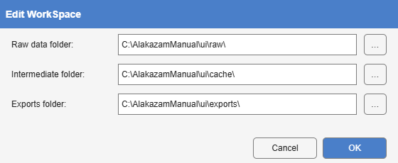
Run startAlakazam from the repository root (Chapter 2). On a machine that has never run Alakazam there is no workspace yet, so a Welcome dialog asks for the raw data folder. The field starts blank and OK is refused until you have chosen one: a plausible-looking placeholder would be a worse start than an obviously empty box. The dialog is the same as Edit WorkSpace on the Alakazam tab (Figure 5.2), so you already know where to change it when you move to another study.
Across the top, the ribbon. Four tabs: Alakazam holds the workspace itself (opening, saving, editing it, the experimental design, settings, the view mode, help); Tools holds the analysis steps, grouped in the order an analysis proceeds; Grand Average combines subjects; Export/Report turns results into files and reports. Chapter 5 describes each.
Down the left, three trees. A Data & Analyses node belongs to exactly one recording. A Grand Average is made from many subjects, so nesting it under any one of them would misrepresent it; a Report can summarise the whole sample. Each therefore has its own tree, and the dividers between them can be dragged.
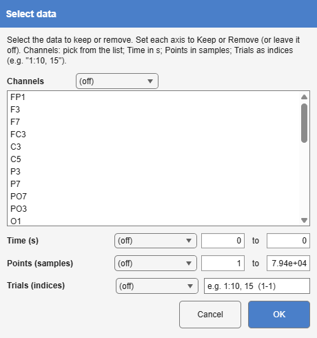
On the right, the plots. One tab per open dataset. The View group on the Alakazam tab switches between Tabs (one at a time), Grid and Stack (all at once, for comparison), and a right-click on a tab can Undock it into a window of its own.
3.4 Opening a recording
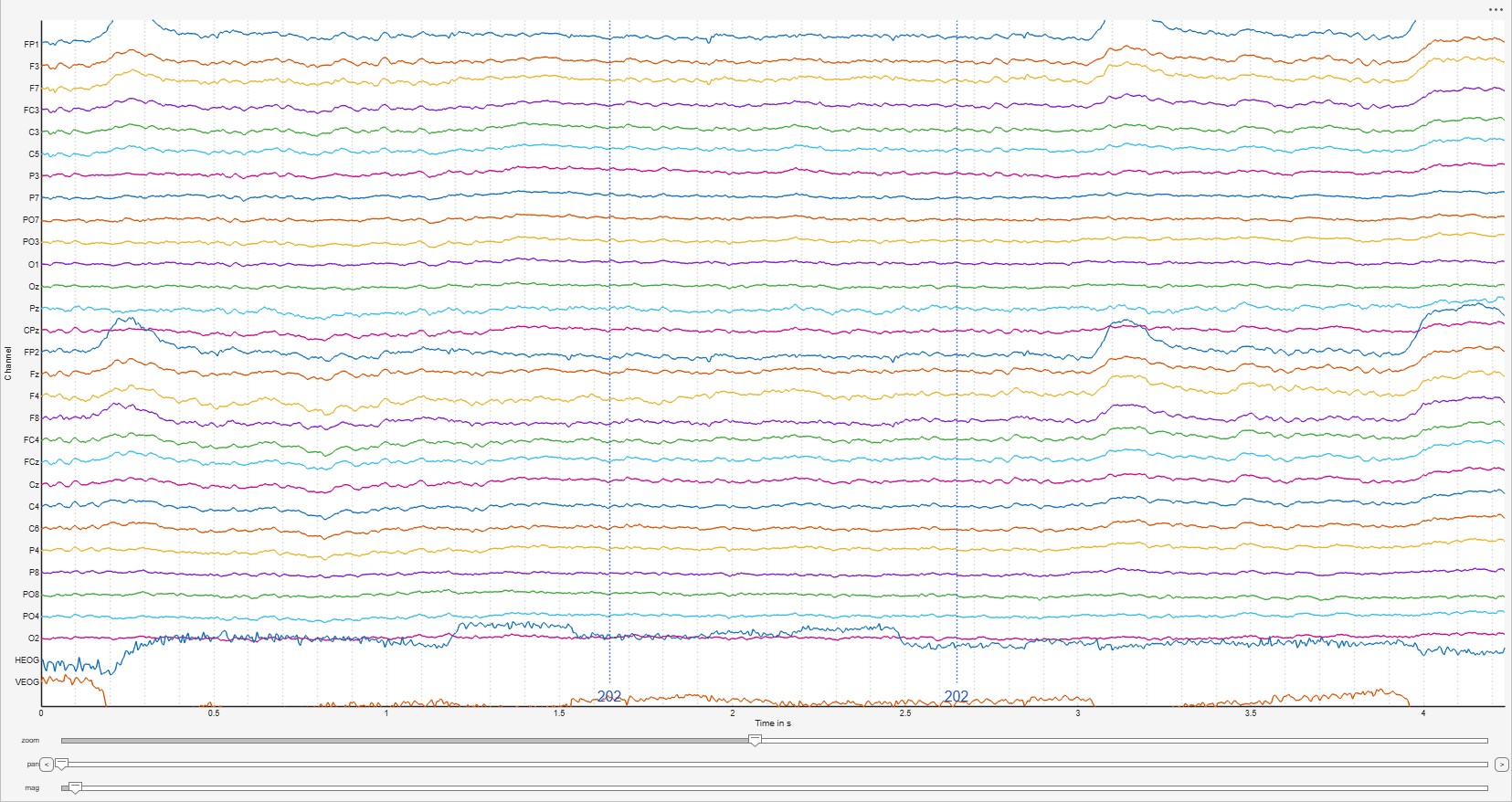
Click a root node in the Data & Analyses tree. A single click loads and draws it; a double click reloads it. Continuous data opens in a scrolling view with the events marked (Figure 3.1). Spend a minute here before doing anything else: check that the events are where you expect them, that no channel is flat, and whether there is drift you will want to filter. Alakazam will compute a clean-looking grand average from bad data, and the cheapest moment to catch bad data is now.
Figure 3.1: A continuous recording (ERP CORE N400, after a 0.1 Hz high-pass filter): channels stacked, events marked as vertical lines with their codes, and the zoom, pan and magnification sliders below.
3.5 Your first transformation
With the recording selected, open Tools > 1. Preprocessing > Filter, set a high-pass filter and confirm. Two things happen, and both matter more than the filter does.
First, a new node appears beneath the recording. The original file has not been touched and will not be. What you are building is a history: the raw recording at the root and each step hanging below the step it was applied to.
Second, the result is written to the Intermediate folder. When you close Alakazam and open it again next week, the filtered dataset is still there, and clicking it is instant.
3.6 The tree branches, and that is the point
Select the filtered node and run another transformation: it lands beneath that node. Now select the raw node again and run something else: a second branch grows from the root. You never choose between two preprocessing routes and lose one. Filter at 0.1 Hz on one branch and 0.5 Hz on the other, run both through to an average, and put the two side by side with Grid. Either the effect survives the choice, which is reassuring, or it does not, which is more important to know (Tanner et al. 2015).
3.7 Doing it again for everybody else
Twenty subjects with six steps each would be a hundred and twenty dialogs. There are three ways out, in increasing order of ambition.
Drag a node onto another recording. Alakazam replays that step, and every step below it, onto the other recording, including branches where the analysis forked. One drag can reproduce a whole pipeline. As a special case, dropping one averaged dataset onto another overlays the two plots instead of transforming anything, as Overlay on plot in its right-click menu does: the quickest way to compare two conditions or two subjects on the same axes (Section 5.4.4). A drop copies the branch; hold Shift while dropping to move it, which removes the original once its copy is made.
Right-click a node and choose Apply to All Raw Files. The same replay, to every recording in the workspace at once. With the Parallel Computing Toolbox several recordings are processed simultaneously, and their results appear as each finishes.
Right-click and Save Template, then Apply Template later. The pipeline goes into a file, which is what you want when the next batch of subjects arrives, or when a colleague asks what exactly you did (Chapter 19).
3.8 From continuous data to an ERP
Tools > 3. Epoching and Averaging holds the step that turns event codes into conditions and cuts epochs around them, DefineBins (Section 9.1), and Average (Section 9.2). Along the way you will usually apply a Baseline correction and some artefact handling, either threshold-based rejection with ArtefactDetect or one of the correction methods in 2. Artifact Rejection / Reduction.
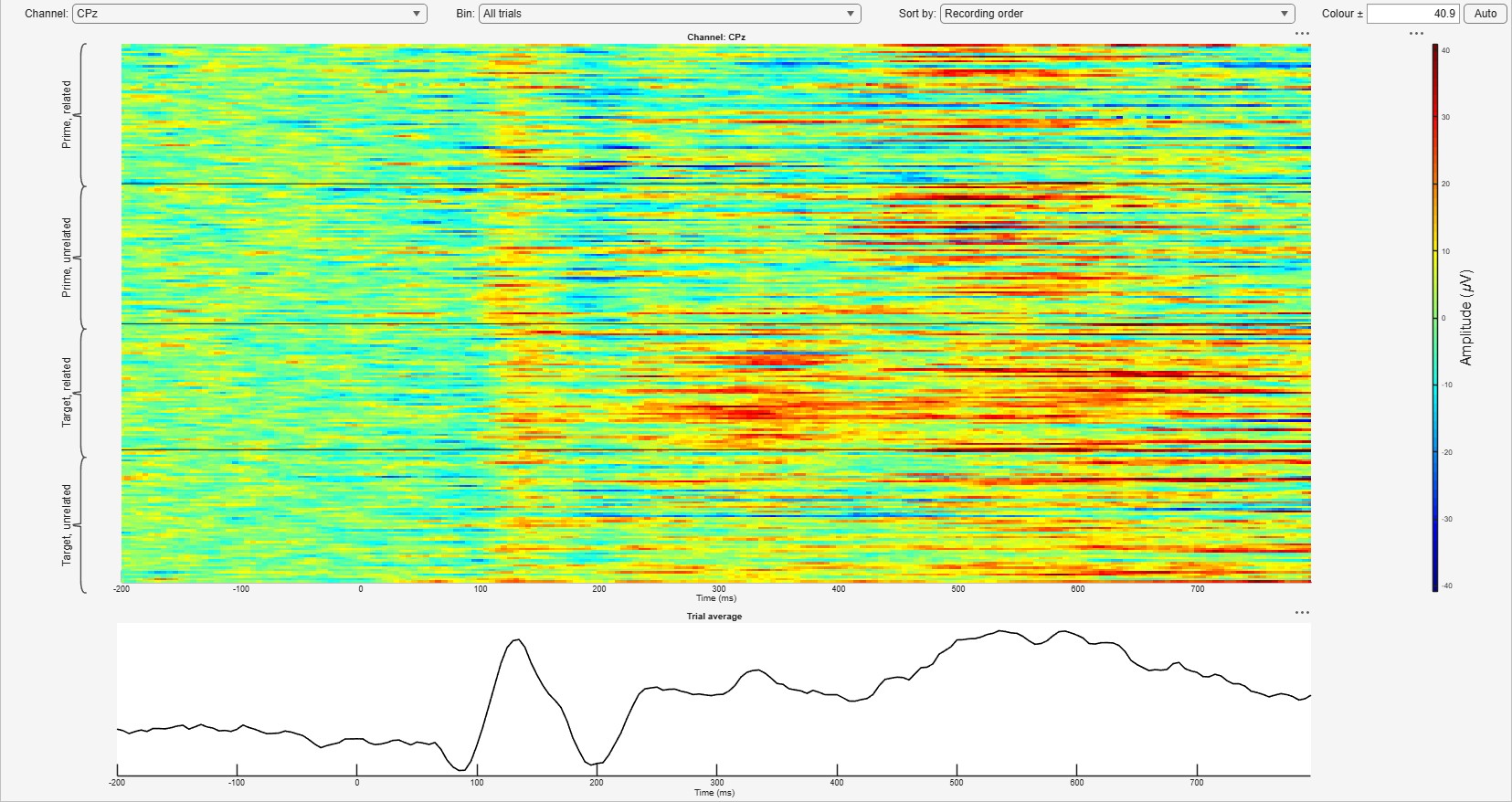
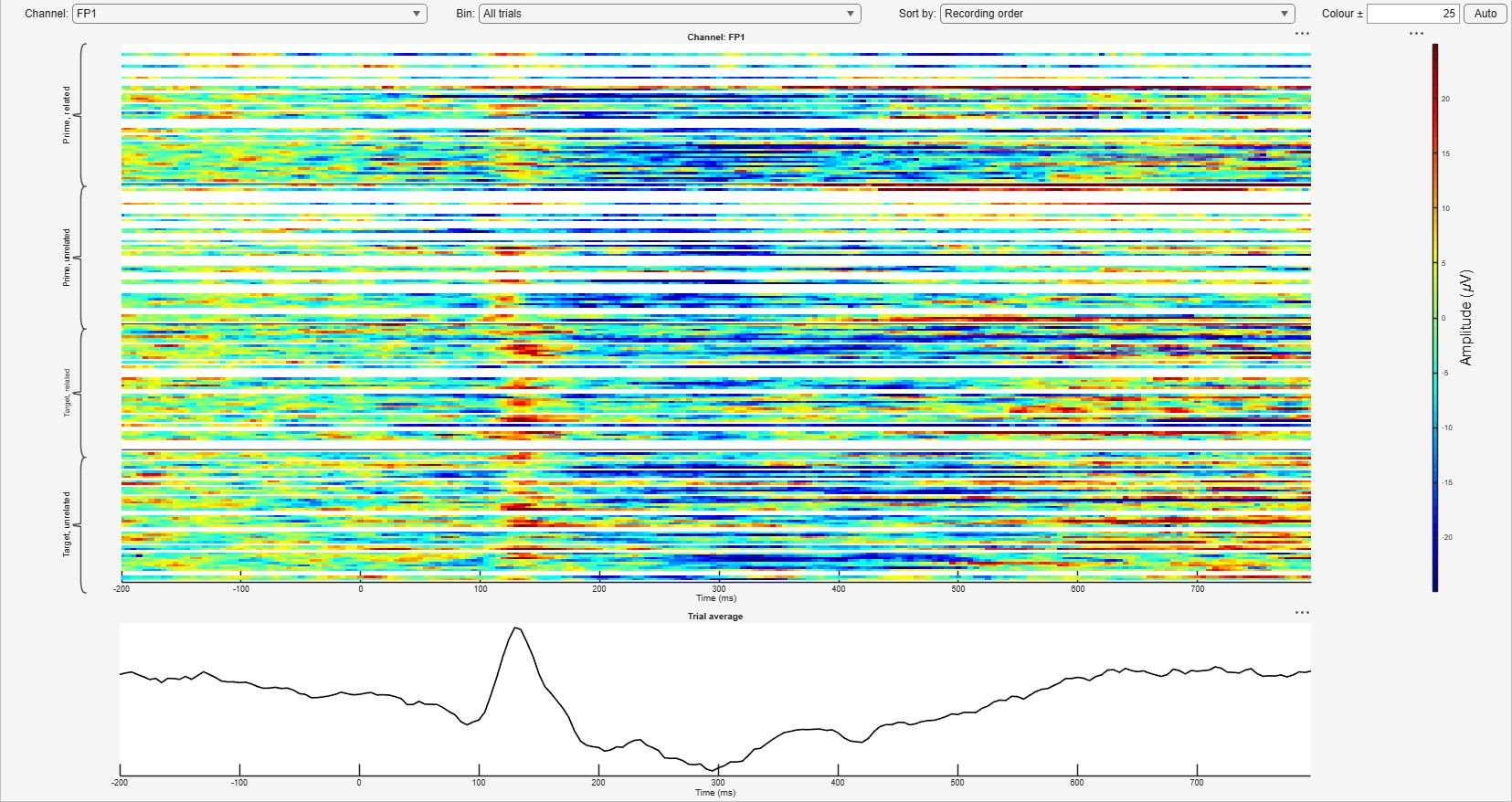
Figure 3.2: The epochs DefineBins cut from the filtered N400 recording, as an ERP image at CPz: one row per trial, grouped by bin, with the average of all trials below.
The order of these steps matters, and in places it is a contested question rather than a matter of taste. The principle that settles most of it is Luck’s: linear operations (filtering, re-referencing, baseline correction, averaging) commute and may be done in any order, whereas non-linear ones (artefact rejection, and correction by ICA) do not, and have to come where their input is what they assume it to be (Luck 2014b). The worked examples give a defensible order for each common paradigm.
3.9 Combining subjects, and getting numbers out
Once several subjects have an average, the Grand Average tab combines them (Chapter 12), and the result appears in its own tree. To get from waveforms to numbers, run ERP Measure (Section 10.1) to say which windows, channels and measures you care about, then use Export/Report > ERP & Report. It writes a CSV and, beside it, a report that runs the test your design calls for rather than a generic one, with the results written out in prose (Chapter 13).
A rendered report gets a node in the Reports tree and opens inside the application. It carries its own copy of the CSV it was built from, so it stays reproducible even if you later overwrite the export.
3.10 Saving, and what “saved” means here
Nothing about the workspace is written to disk automatically. Save WorkSpace on the Alakazam tab records your three folders, the last settings of every transformation you have run, and the design (groups, persons, sessions). Your results look after themselves: they are in the Intermediate folder as soon as they are computed. Deleting that folder costs computation time and nothing else, which is why Clear WorkSpace is safe to use when an analysis has become a tangle.
4 Concepts
This chapter describes the ideas the rest of the manual assumes: what a workspace is, what a node in the tree holds, the three shapes a dataset can have, and the ways a pipeline is replayed.
4.1 Workspaces
A workspace is the three folders of Table 3.1 together with a small amount of state: the last options of every transformation, and the design (which recordings belong to which group, person and session). It is stored as a .wksp file, a small JSON document:
The ~ stands for the user’s home folder, which keeps a workspace portable between machines. Opening a workspace scans its raw folder and rebuilds the tree from the cache; nothing is recomputed.
Nothing about a workspace is saved automatically: Save WorkSpace is the one moment its state is written. Results are a different matter, since each is written to the cache as it is computed.
4.2 The tree and its nodes
Each recording is a root node. Applying a transformation to a node produces a child node holding the result, so the tree records, for every result, the chain of steps that produced it. A node’s context menu (right click) offers what can be done with that node:
Table 4.1: A node’s context menu. Actions a node cannot perform are shown disabled.
Action
What it does
Recalculate
Reopen the step’s dialog with the options it was run with, and recompute it and everything below it.
Apply to All Raw Files
Replay this node’s branch on every other recording in the workspace.
Save Template / Apply Template
Write the branch to a template file; replay a template here.
Rename, Delete
Rename a node, its open plot taking the new name too; delete it and its branch, and the files behind them.
List events
Count the event codes in a dataset.
Overlay on plot
Draw an average on the ERP plot in view, or a continuous recording under the continuous recording in view, to compare the two (Section 5.4.4, Section 5.4.1.1).
Rejection breakdown
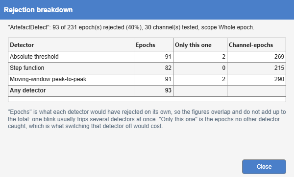
For an ArtefactDetect node: which detector rejected which trials (Figure 8.3).
Export as ERPset, Export as EEGLAB .set
Hand an averaged dataset to ERPLAB, or any dataset to EEGLAB.
Recalculate is offered for every transformation whose dialog can be reopened with the options stored on the node. It is not offered for a raw root, for a step with no options (Average, Scalp, Brain), or where reopening the dialog would not mean what it meant the first time:
EventEditor and Photodiode open on the dataset’s own events and signal, and do not read stored options.
ICA (RemoveComponents) stores component numbers, and a new decomposition numbers its components differently, so the stored choice could remove the wrong ones.
ManualReject, although driven by inspection, can be recalculated: the trials and channels it flagged are the same trials and channels when its input is recomputed, so its dialog reopens with them flagged.
4.2.1 What a node records
Each node holds a complete EEGLAB dataset, plus a record of how it was made: the transformation’s name and the options it used. Where a step changes what the numbers mean without changing how they look, it also records what it did: which channels it interpolated in which trials, which artefact detector rejected which trial, which ICA components it removed, which channels it rectified and how, the model a deconvolution fitted. The data-quality report (Chapter 15) reads these records, so that a subject whose data were heavily interpolated cannot pass as a clean one.
4.2.2 The cache
A node’s result is a file in the workspace’s Intermediate folder, in a subfolder named after its recording. Beside each result are two small records (.json and .meta) that let Alakazam build the tree and replay a branch without loading the data. Deleting the cache costs recomputation and nothing else; Clear WorkSpace does it for one workspace’s recordings, either keeping each recording’s imported copy (normal) or not (deep), and never touching another workspace that shares the folder.
4.3 The shapes of a dataset
A dataset has one of three formats, and which transformations apply to it follows from which:
Table 4.2: The three dataset formats.
Format
Shape
Produced by
Viewed as
Continuous
channels × samples
import, preprocessing
a scrolling signal view
Epoched
channels × samples × trials
DefineBins with an epoch window
an ERP image
Averaged
channels × samples × bins
Average, Deconvolve, Grand Average
ERP waveforms
Frequency-domain results (Fourier, Welch) keep the format of their input and change the axis from time to frequency.
4.3.1 Bins
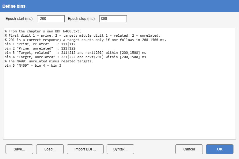
A bin is a condition: the set of events that belong together, and the epochs cut around them. Bins are defined with DefineBins’ small language (Section 9.1), which can select events by their codes and by their relations to neighbouring events (a target followed by a correct response within 200 to 1500 ms, for instance). An event can belong to several bins.
A combination bin is arithmetic on other bins, such as bin 5 = bin 4 - bin 3 for a difference wave. It has no events of its own: Average computes it from the bins it names, and its standard error from theirs.
4.4 Replaying a pipeline
A pipeline built on one recording can be applied to others in four ways, all of which replay the stored options rather than reopening the dialogs:
Drag and drop a node onto another recording: that step and every step below it, including forks, are replayed there.
Apply to All Raw Files: the same, onto every recording in the workspace, in parallel when the Parallel Computing Toolbox is installed.
Templates: a branch written to a .alztemplate file and applied later, in any workspace.
Export as Code: the whole workspace written as a MATLAB script (Section 19.4).
Options are stored by channel and bin label, not by position, so a pipeline replays correctly on a recording whose channels are in a different order, and one that lacks a stored channel says so rather than computing on the wrong one.
4.5 Grand averages and reports
A grand average combines several subjects’ averages into one, in its own tree (Chapter 12). A report is a rendered Quarto document, statistical, cluster-based or about data quality, with its own node in the Reports tree and its own copy of the data it was computed from (Chapter 13, Chapter 15).
Both trees show only what belongs to the open workspace. Several workspaces may share one Cache or Exports folder, so a grand average is listed where the recordings it was built from are, and a report where it was rendered: each report records the Raw folder of the workspace that made it. A report rendered before reports kept that record is listed where its tables name a recording of the workspace, and everywhere when they name none.
5 The interface
This chapter is a reference to the window: the four ribbon tabs, the trees, the plot area and the controls each kind of plot offers, and the settings that apply to all of them.
5.1 The ribbon
The ribbon has four tabs. A button that cannot act on the current selection is disabled rather than hidden, so the layout never shifts.
5.1.1 Alakazam
Figure 5.1: The Alakazam tab.
Table 5.1: The Alakazam tab.
Group
Button
Action
Workspace
Open WorkSpace
Load a .wksp file: its folders, the last options of every transformation, and the design.
Save WorkSpace
Write the same to a .wksp file. The only moment workspace state is saved.
Figure 5.2: Edit WorkSpace: the three folders of a workspace, each with a folder browser.
5.1.2 Tools
Figure 5.3: The Tools tab. A group whose buttons do not fit shows a more count and opens a menu with the rest.
The Tools tab holds every transformation, grouped in the order an analysis usually proceeds. The groups are the chapters of the reference part of this manual:
The ribbon is built from the transformations it finds at startup, so a transformation added to the source tree appears without further configuration (see the developer guide).
5.1.3 Grand Average
Figure 5.4: The Grand Average tab.
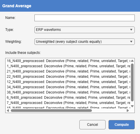
Define Grand combines subjects’ averages into one; Per Design Cell makes one grand average for every cell of the design (each group, for instance) at once; Export Grand writes every grand average’s waveforms to a CSV. Chapter 12 describes all three.
5.1.4 Export/Report
Figure 5.5: The Export/Report tab.
Table 5.3: The Export/Report tab.
Group
Button
Action
Batch Export
ERP & Report
Collect every ERP Measure result into one CSV, and write the statistical report (Chapter 13).
Spectral & Report
The same for Spectral Measure results (Chapter 16).
Cluster Statistics
Cluster Test
A cluster-based permutation test over channels and time (Chapter 14).
Source Cluster
The same test over the cortical surface (Section 14.4).
Data Quality
Data Quality Report
Trial loss, noise and measurement error per subject and condition (Chapter 15).
Reproducibility
Export as Code
The whole workspace as a MATLAB script (Section 19.4).
5.2 The trees
The three trees on the left hold results of three different kinds:
Data & Analyses: one root per recording, and below it every transformation applied to it (Section 4.2).
Grand Averages: results combined over subjects, which belong to no single recording.
Reports: every rendered report, which opens inside the application.
Selecting a node in one tree clears the selection in the other two, so there is never doubt about which dataset a ribbon button will act on. A single click on a node draws it; a double click forces it to be read from the cache again. The dividers between the trees can be dragged.
A node’s icon says what it holds: a person for a raw recording, a waveform for a time-domain result, bars for a frequency-domain result, and a fan for a grand average. Its right-click menu is described in Table 4.1.
5.2.1 Dragging nodes
Dragging a node onto a recording’s root replays the step, and every step below it, onto that recording (Section 4.4). Dragging an averaged dataset onto another averaged dataset of the same shape does not transform anything: it overlays the first on the second’s plot, the same as Overlay on ERP plot in its right-click menu (Section 5.4.4).
A drop copies: the original branch stays where it was. Hold Shift while dropping to move it instead, and the cursor shows a move while Shift is held. The branch is replayed onto the new dataset as before, since its results depend on the data under it, and the original is then deleted, its files and any open plots with it, as Delete would. What counts is Shift at the moment of the drop. The original is kept, with a note saying why, when a grand average was made from one of its datasets (it would be left without them; copy the branch, or define the grand average again first), when the drop was an overlay, or when the branch could not be replayed in full.
5.3 The plot area
Each dataset that is drawn gets a tab in the plot area. The View group on the Alakazam tab chooses how the tabs are shown:
Tabs: one plot at a time.
Grid: every open plot at once, in a grid.
Stack: every open plot at once, one above the other.
Right-clicking a plot’s tab offers Undock, which moves the plot into a window of its own (for a second monitor); its tab remains, with a Dock button, and closing the window puts the plot back. Close and Close others close plots; closing a plot discards nothing, and selecting the node again reopens it.
5.3.1 The channel and bin follow you
When a new plot opens, it shows the channel that was showing in the plot before it and, in every view that shows one bin at a time, the bin as well. Stepping down a branch from filter to epochs to average therefore keeps showing Pz, rather than returning to the first channel at every step. The match is by label, so it holds when the channels are in a different order or some are missing; a dataset without that channel keeps its own default. This is a convenience of the session and is not saved.
5.4 Plot types
Which view draws a dataset follows from its format (Table 4.2) and the transformation that made it.
5.4.1 Continuous data
Figure 5.6: Continuous data: the channels stacked, events as labelled vertical lines, a scroll bar that pages through the channels on the right, and the pan, zoom and magnification sliders below.
Continuous data is drawn by a renderer that precomputes a pyramid of per-bucket minima and maxima, so that a redraw reads about one value pair per screen pixel, whatever the length of the recording. Because minima and maxima combine exactly, the decimated trace never hides a spike or a brief artefact, which a plotting routine that subsamples would.
Table 5.4: Controls of the continuous view.
Control
Action
pan slider, mouse wheel
Move through time.
zoom slider
The length of time shown.
mag slider
The amplitude scale.
Vertical slider (right)
Page through the channels, when there are more than fit legibly.
Events are drawn as vertical lines with their codes; intervals marked by artefact detection are shaded. Zoomed in until every sample has two pixels or more to itself, that is with fewer samples in view than half the plot’s width in pixels, each sample is marked with a small filled circle, which shows where the signal was measured and where the line only joins the dots.
Each channel starts at its label on the left: its value at the left edge of the view is taken off before it is drawn, so slow drifts and DC offsets do not carry the traces across the screen as you zoom and scroll, and mag magnifies each trace about that point. This is display only; the data are not changed. Turn View-on-screen baseline off (Section 5.5) to centre each channel on its row by its median over the whole recording instead.
5.4.1.1 Overlaying a recording
To see what a step did to the raw signal, show the recording after the step, then right-click the recording before it (or any other continuous node) and choose Overlay on plot. It is drawn underneath as a grey ghost, each of its channels in the lane of the channel with the same name and at the same magnification, while the channels of the plot keep their colours. Its own time axis is used, so a resampled recording lines up with the original; two recordings with no channel in common, or that do not overlap in time, are refused with the reason. Dragging is not an overlay here: dropping a continuous node onto another replays its steps (Section 4.4).
A row of controls appears under the sliders while a recording is overlaid: which recording it is, opacity (how dark the ghost is), Difference and Remove overlay. Difference draws, in each lane, the plot’s recording minus the overlaid one, which is what a filter or a cleaning step removed; a channel the overlaid recording lacks is left empty. The difference is worked out from the raw samples in view, so zoomed out over a long recording it asks to be zoomed in first. One recording is overlaid at a time: overlaying another replaces it.
5.4.2 Epoched data: the ERP image
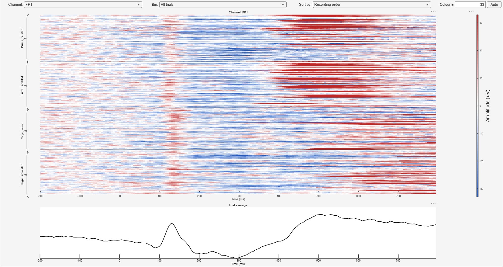
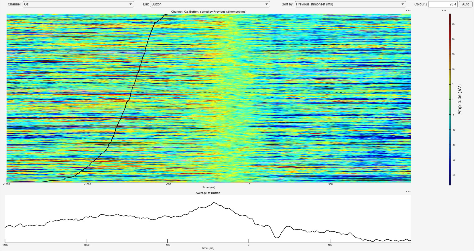
Figure 5.7: The ERP image of an epoched dataset at one channel: one row per trial, colour for amplitude, grouped by bin, and the trial average below.
Epoched data is drawn as an ERP image (Jung et al. 2001): one row per trial, time across, colour for amplitude, with the average of the shown trials below. The up and down arrow keys, or the mouse wheel, step the channel.
Table 5.5: Controls of the ERP image.
Control
Action
Channel
Jump to a channel.
Bin
Show one bin’s trials only, with their average below; or all.
Sort by
Order the rows by a value each trial carries (below).
Colour ±
The colour range for this channel’s type (EEG, EOG, other); Auto takes the 98th percentile of the absolute amplitude.
Sort by orders the trials by a value each one carries: the time to the next or the previous event of any type (Next saccade, Previous stimonset), measured when the trials were cut; the reaction time DefineBins captured for the trial’s bin; or any numeric field of the trial’s own event, such as a fixation’s duration or a saccade’s amplitude from an eye tracker. When the value is a time, it is drawn across the image as a line. That line is how overlapping activity is told from a response: activity locked to the time-locking event runs straight down the image, while activity that belongs to the next event bends with the line (Chapter 17).
The smallest value is at the top, or the largest with Reverse the sort (Section 5.5); trials without a value go last. With Plot trials by bin on, the sort happens within each bin. Rejected trials are drawn blank.
5.4.3 Averaged data: ERP waveforms
Figure 5.8: Averaged data: one line per bin at the chosen channel, each with its confidence band, and a tick box per bin on the right.
An averaged dataset is drawn as one waveform per bin, each with a band of n standard errors of the mean around it (the width is set in Section 5.5). The tick boxes on the right show and hide bins; the up and down arrow keys, or the mouse wheel, step the channel for every line at once. When the dataset carries ERP Measure results, the measurement windows are drawn on the waveforms: the window shaded, and the measured value marked (a peak, a fractional latency, or the area filled).
Dragging the plot, and the toolbar’s pan and zoom, move or scale the amplitude axis only; the time axis stays as drawn. Dragging is how to put zero where you want it. What a zoom or pan sets is kept for every channel while you step through them, and while you tick lines, so all electrodes are seen at the scale and offset you chose; the toolbar’s Restore view returns to automatic scaling. The difference (below) keeps its own amplitude zoom.
5.4.4 Overlaying ERPs
Two subjects, two conditions, or the same average before and after a preprocessing step are easiest to compare on the same axes. Show one ERP, then right-click another averaged node, in either tree, and choose Overlay on plot: its waveforms are added to the ERP plot in view (the selected tab, or in a grid the tile last clicked). Dragging one average onto another does the same.
Channels are matched by name, and each line keeps its own time axis. A resampled average overlays the original, and so does one with a different montage or channel order: every line shows the electrode named in the title, and a dataset without that electrode says so in its tick box. Two datasets with no channel in common, or with time ranges that do not overlap, are refused with the reason. Only averages drawn as waveforms can be overlaid; a scalp map or a time-frequency result cannot. Spectra are overlaid in the same way on the spectrum view (see Spectra, below).
Lines are named by what sets their datasets apart in the tree: two subjects’ averages read S01 and S02, two branches of one subject by the step where they part. Nodes carry their transformation’s name until they are renamed, so two branches whose nodes are all called the same are told apart as [1] and [2], the plot’s own dataset first; renaming a node (right-click, Rename) gives its lines a clearer name. The full path is in the tick box’s tooltip.
Overlaid datasets are drawn underneath and paler than the plot’s own, so its lines stay readable; Overlay opacity, below the tick boxes, sets how pale. Remove overlay takes every overlaid dataset off the plot again and leaves its own lines as they were.
Difference. With exactly two lines ticked, Difference draws the first minus the second instead of the two lines, and Swap reverses the subtraction: the difference between two bins of one average, or what a filter removed from the same bin. When the two were sampled differently, the second is interpolated onto the first’s time points. No confidence band is drawn around a difference: the two lines may share their trials, as the same bin before and after a filter does, and then the standard error of their difference cannot be derived from theirs. For a difference with its own error, define a difference bin (Section 9.1).
An overlay is part of the plot, not of the workspace: closing the plot removes it.
5.4.5 Spectra
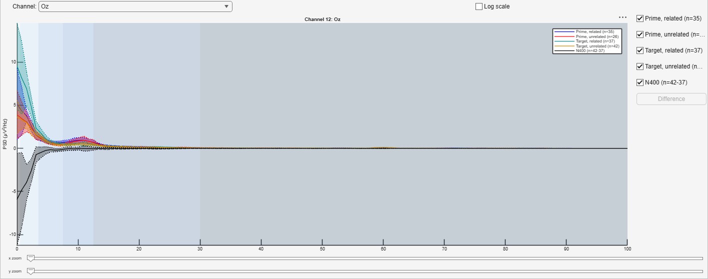
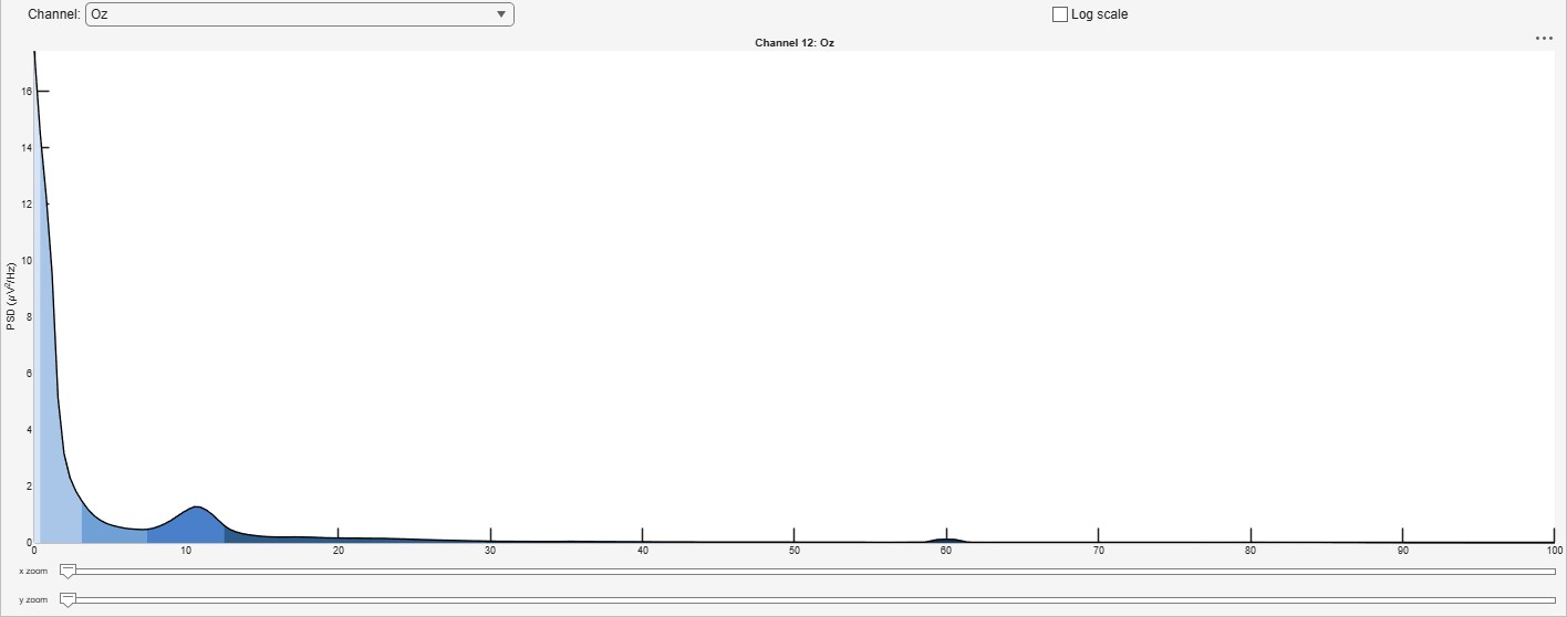
A frequency-domain result (Fourier, Welch) is drawn as a spectrum, with the named frequency bands of Section 5.5 shaded: filled under the curve when one spectrum is drawn (from 0, or from the bottom of a log axis), and as pale stripes behind the lines when there are several, or a difference, since there is then no one curve to fill under. Above the plot are the channel and the log scale; below it, two sliders zoom.
An averaged spectrum overlays its bins, as the ERP plot does (Section 5.4.4): a tickbox for each bin beside the plot, each ticked bin a line in the same colour it has in the ERP plot, and, where Average stored it, a band of standard errors, set by the ERP plot’s own Show confidence interval settings. With exactly two bins ticked, Difference draws the first minus the second (Swap reverses it). Ratio in dB draws their ratio in decibels instead: 10·log10 of it for a power, 20·log10 for an amplitude. The ratio is the usual way to compare conditions in a spectrum, since it does not depend on the overall level, which falls steeply with frequency. With the phase shown (P), the difference is the phase of the first bin relative to the second.
Other spectra can be overlaid exactly as ERPs are (Section 5.4.4): show one spectrum, then right-click another averaged spectrum, or a Welch spectrum of a continuous recording, and choose Overlay on plot; dragging one averaged spectrum onto another does the same. Channels are matched by name and each spectrum keeps its own frequencies, so one of another resolution or montage overlays the original. Overlaid lines are named, drawn underneath and paler, and taken off again, as on the ERP plot, and Difference and Ratio in dB compare any two ticked lines, of one dataset or two, interpolating the second onto the first’s frequencies. A spectrum in another unit (power on amplitude, say) cannot share the axis and is refused with the reason, and so are single-trial spectra. Overlaying two Welch spectra is the quickest way to see what a cleaning step removed, or how two recordings differ at rest.
The single-trial spectra of an epoched recording are shown one at a time, picked by trial, and take no overlay; average them to compare bins.
Table 5.6: Controls of the spectrum view.
Control
Key
Action
Channel
up, down
The channel shown. The mouse wheel also steps through the channels.
Trial
left, right
The trial of an epoched spectrum, with the bin it belongs to.
Tickboxes
The lines drawn: the bins of an averaged spectrum, and those of an overlaid one.
Difference, Swap, Ratio in dB
Compare two ticked lines.
Remove overlay, Overlay opacity
Take the overlaid spectra off, or set how pale they are drawn.
Log scale
Draw the magnitude on a logarithmic axis, six decades deep. Off by default; not for a phase, a difference or a ratio.
x zoom, y zoom
Zoom the frequency and power axes.
P
Switch between magnitude and phase, for a complex spectrum.
The x zoom is anchored at the left edge of the window, so that 0 Hz stays in view unless the axis has been panned with the plot’s toolbar. On a log scale the y zoom keeps the bottom of the axis and brings its top down.
5.4.6 The other views
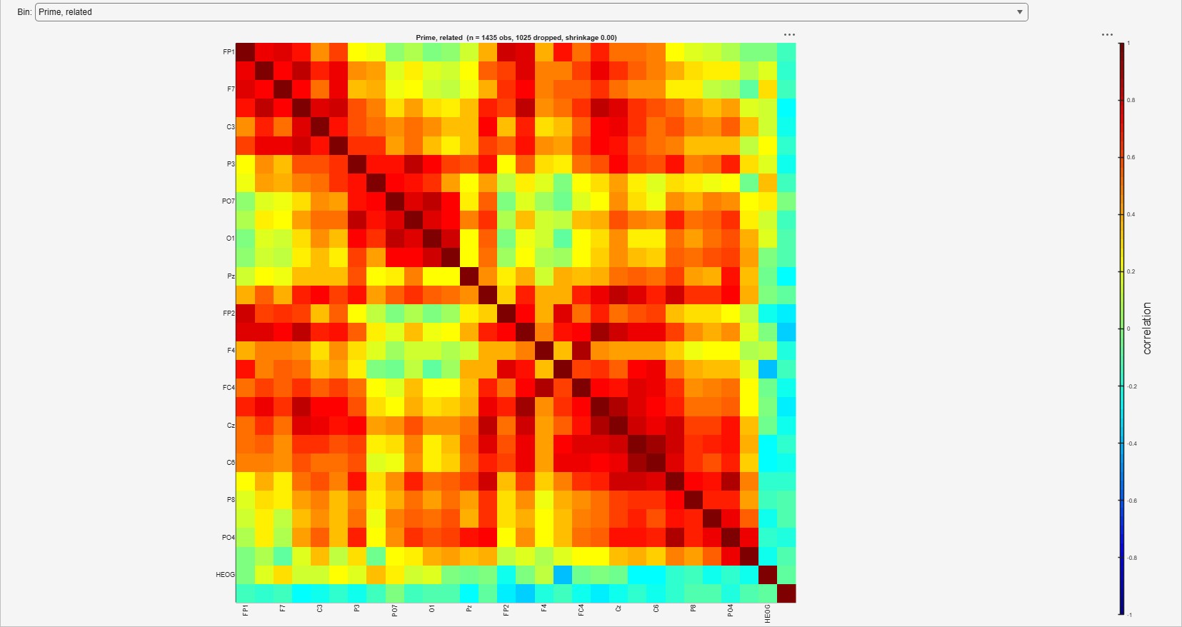
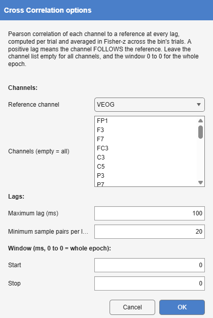
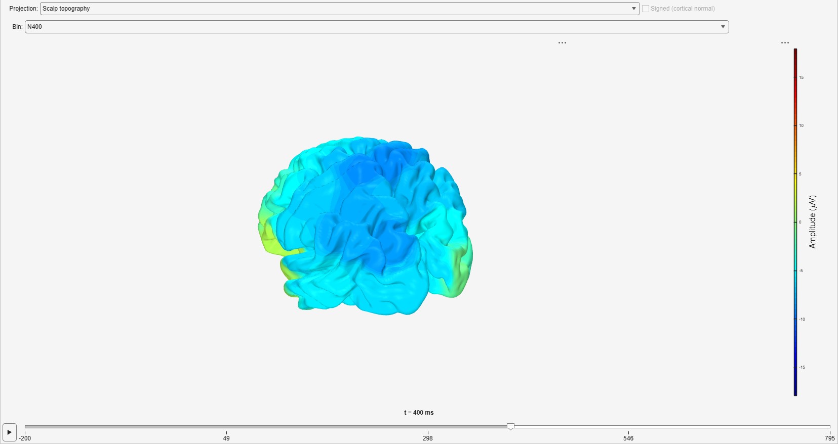
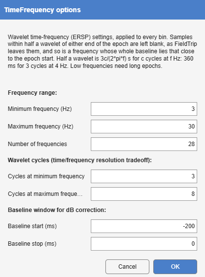
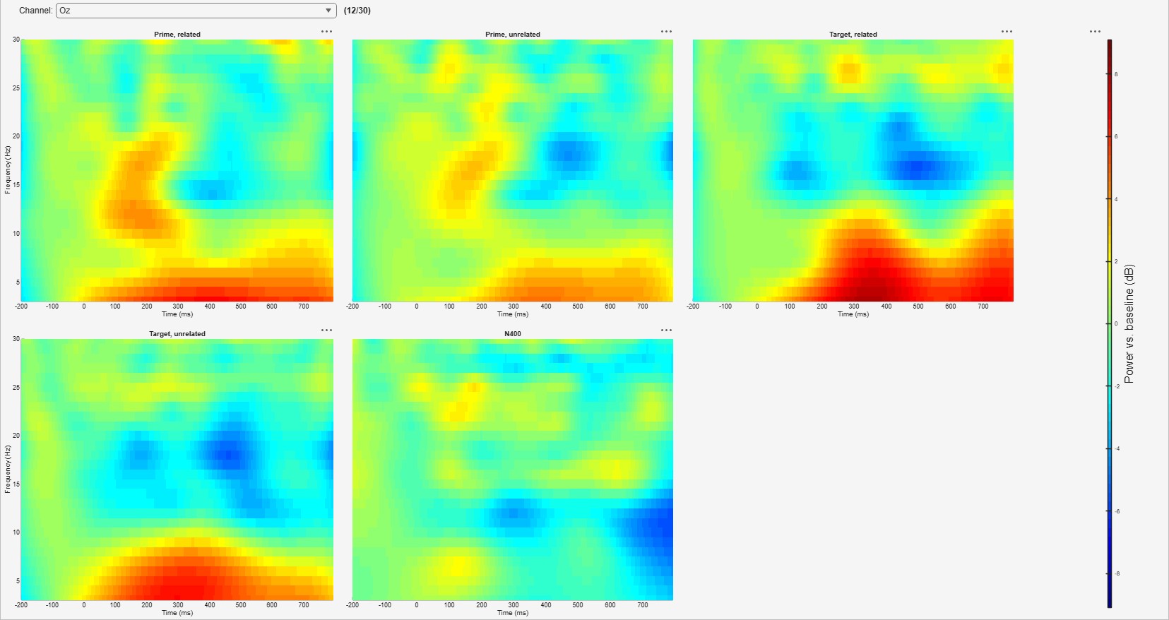
Scalp maps and the 3D brain have a bin menu, a time readout, a slider that scrubs through time and a Play button; the map redraws as the slider moves. Time-frequency, coherence, covariance and cross-correlation results have their own views, described with the transformations that produce them in Chapter 10 and Chapter 11.
5.5 Settings
Alakazam > Settings > Global opens the preferences. They apply to every workspace, and Save writes them at once, to a preference file that is separate from any workspace.
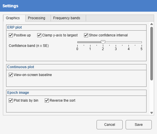
Figure 5.9: Graphics
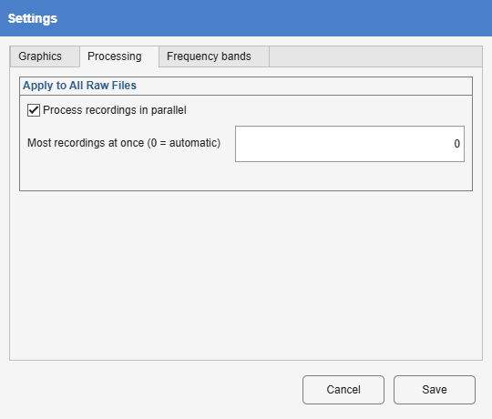
Figure 5.10: Processing
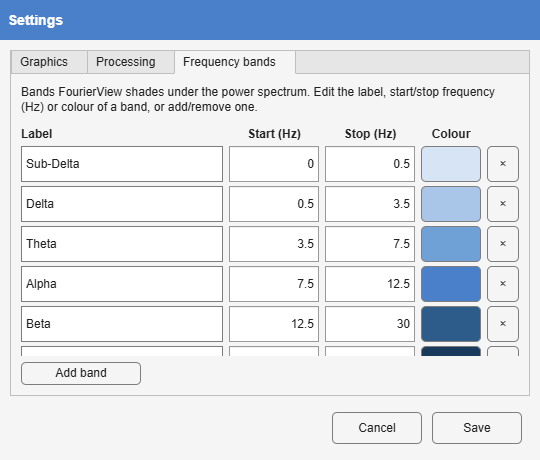
Figure 5.11: Frequency bands
The three tabs of the settings dialog, as set on the machine that made this manual’s figures (which differs from the defaults of Table 5.7 in the clamped y-axis, the band width, and the ERP image’s grouping and sort order).
Table 5.7: The global settings.
Tab
Setting
Default
Effect
Graphics
Positive up
on
ERP polarity. Off draws negative up, the convention of much of the older literature.
Clamp y-axis to largest
off
One y range for every channel, taken from the largest, so that amplitudes can be compared across channels by eye. Off rescales per channel.
Show confidence interval, Confidence band
on, 3
The band around each waveform, in standard errors of the mean.
View-on-screen baseline
on
Each channel of a continuous recording starts at its label at the left edge of the view, whatever the zoom and scroll. Off centres it on its row by its median over the whole recording.
Plot trials by bin
off
Group an ERP image’s rows by bin; a trial in two bins then appears twice.
Reverse the sort
off
Put the largest sort value at the top of the ERP image, as EEGLAB’s erpimage does.
Colour map
diverging
The map of every signed, zero-centred plot: ERP image, time-frequency power, scalp maps. diverging is a blue-white-red scale centred on zero; the alternatives are MATLAB’s parula, jet, turbo, hot and cool.
Smooth spectrum
off
Smooth a spectrum with a light moving average before drawing it. The data are not changed.
Processing
Process recordings in parallel
on
Whether Apply to All Raw Files uses parallel workers, when the Parallel Computing Toolbox is installed.
Most recordings at once
0
The number of workers; 0 takes the smallest of the number of recordings, the physical cores and what free memory allows for the largest recording.
Frequency bands
label, start, stop, colour
sub-delta to gamma
The bands shaded beneath a spectrum: sub-delta 0 to 0.5 Hz, delta 0.5 to 3.5, theta 3.5 to 7.5, alpha 7.5 to 12.5, beta 12.5 to 30, gamma 30 to 100.
A zero-centred diverging map is the safer choice for signed data: zero is white, and the sign of an effect is read from the hue rather than from a position along a rainbow. Rainbow maps such as jet introduce apparent boundaries that are not in the data (Borland and Taylor 2007).
6 Your data and your design
This chapter covers what Alakazam reads, how a workspace is set up and cleaned, and how the design of a study (groups, persons and sessions) is declared so that grand averages and the statistical reports can use it.
6.1 File formats
Every file directly inside the raw folder becomes a root node. The format is recognised by its extension:
Table 6.1: File formats read from the raw folder.
Extension
Format
Arrives as
Notes
.set (with .fdt)
EEGLAB dataset
continuous or epoched
Read with EEGLAB’s pop_loadset.
.vhdr (with .eeg, .vmrk)
BrainVision
continuous
Read with the bva-io plugin, installed on first use.
.erp
ERPLAB erpset
averaged
Read directly, without ERPLAB; a root at the ERP stage, so only ERP-domain steps apply.
.mat
an Alakazam dataset
as saved
A dataset saved by Alakazam or exported from its cache.
.edf
European Data Format (EDF, EDF+)
continuous
BIOSIG. Labels such as EEG Fp1-REF need renaming to 10-5 labels for positions.
.bdf
BioSemi
continuous
BIOSIG. Recorded without a reference: re-reference first.
.gdf
General Data Format
continuous
BIOSIG.
.cnt
Neuroscan or ANT Neuro
continuous
The Neuroscan reader, or File-IO for an ANT file.
.mff (a folder)
EGI Netstation
continuous
The mffmatlabio plugin; event types from each event’s code.
.raw
EGI simple binary
continuous
EEGLAB’s own reader.
.xdf
Lab Streaming Layer
continuous
The xdfimport plugin; the EEG stream, with the other streams’ markers as events.
.trc
Micromed
continuous
File-IO.
.e
Nicolet
continuous
File-IO.
.fif
MNE-Python / Neuromag
continuous
File-IO; every channel is read, so select the EEG with SelectData.
The first four have always been read; the others go through the reader named, an EEGLAB plugin that EEGLAB’s plugin manager installs the first time a recording needs it, with EEGLAB’s File-IO route (FieldTrip’s readers) as the fall-back when that reader is missing or refuses the file. Which reader made the dataset is kept with it. Two extensions are not read, because a file with them could be one of several things: .eeg (BrainVision’s data file, opened through its .vhdr, but also Nihon Kohden’s and Neuroscan’s) and .dat. Such a recording can be read with its own EEGLAB reader and saved as a .set. A recording that cannot be read does not stop the workspace from opening: it is left out of the tree, and one message lists every such file and why.
The first time a recording is opened, it is read and its imported copy written to the cache; later openings read the copy, unless the raw file has become newer, in which case it is read again. An EyeLink file (.asc, or .edf when SR Research’s converter is installed) is not a recording in its own right: it lies beside the recording it belongs to and is joined onto it by the eye-tracking step (Section 7.4). An EyeLink .edf is told apart from a European Data Format one by its first bytes, and left alone.
6.1.1 What Alakazam expects of a recording
Channel labels. Interpolation, ICA and the source estimates need electrode positions. When a recording carries positions they are used as they are; when it carries only labels, positions are looked up in the 10-5 template by label. Scalp maps always place a channel by its label on the 10-5 template, so a channel whose label is not a 10-5 name is left out of them. ChannelEditor (Section 7.1) sets or corrects labels and positions.
Channel types. A channel is taken to be peripheral rather than scalp EEG when its type, or failing a type its label, says so: EOG, HEOG, VEOG, ECG, EMG, EYE, a photodiode, a trigger channel and similar. Peripheral channels do not set the colour range of scalp maps, have their own colour range in the ERP image, are excluded by the “scalp EEG only” choices of artefact detection, and are left out of ICA.
Event codes. DefineBins reads the event type field. Numeric codes and strings (S 12, stim/face) both work; the bin language matches them with wildcards (Section 9.1).
6.2 Setting up a workspace
A workspace is set up with Edit WorkSpace (Figure 5.2), or by writing its .wksp file directly (Section 4.1). Changing the raw folder rescans it and rebuilds the tree at once. Save WorkSpace records the folders together with the last options of every transformation and the design; Open WorkSpace restores all three.
A cache folder can be shared by several workspaces: each recording’s results live in a subfolder named after it, and a workspace touches only its own recordings’ subfolders.
6.3 Cleaning a workspace
Clear WorkSpace asks for one of two levels:
Normal removes every transformation result of every recording in the workspace, and every grand average built only from them, but keeps each recording’s imported copy, so reopening a recording stays quick. This is the one to use before rerunning a revised pipeline.
Deep also removes the imported copies, so that every recording is read again from its raw file.
Either way the raw recordings are left alone, as are other workspaces’ recordings in a shared cache. The operation cannot be undone.
Clear Other keeps one recording’s branch (the selected root) and removes every other recording’s results: the usual step before replaying a revised pipeline from the recording it was developed on.
6.4 Declaring the design
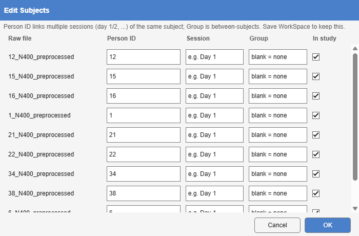
A workspace starts as a within-subjects design: every recording is a different subject, and every bin a condition measured in each. Anything else is declared in Alakazam > Design > Grouping (Figure 6.1), which has one row per recording:
Table 6.2: The columns of Grouping.
Column
Default
Meaning
Person ID
the part of the file name that differs between recordings
Recordings with the same Person ID are one person measured more than once.
Session
blank
A label for the repeated measurement: Pre, Post, Day 1.
Group
blank
A between-subjects group: patient, control. Blank means no group.
In study
ticked
Unticked takes the recording out of every grand average, report and statistic, and lists it wherever the design is shown.
Figure 6.1: Grouping: one row per recording, with its person, session, group and whether it is in the study.
The Person ID default is found by removing from every file name the parts common to all of them (an experiment name, a suffix such as _preprocessed), since those cannot tell subjects apart.
What each column changes in the statistics:
The random effects of the mixed models are grouped by Person ID, so a person recorded twice counts once.
Session becomes a within-subjects factor, crossed with bin, when the recordings support one: at least two session labels, at least two people measured in more than one session, and no empty cell. When they do not, the report fits the simpler model and says why.
Group turns each test into its between-subjects or mixed counterpart as soon as two different labels are in use (Chapter 13).
Group and session assignments are kept for the session only until Save WorkSpace writes them.
6.4.1 Checking the design before analysing
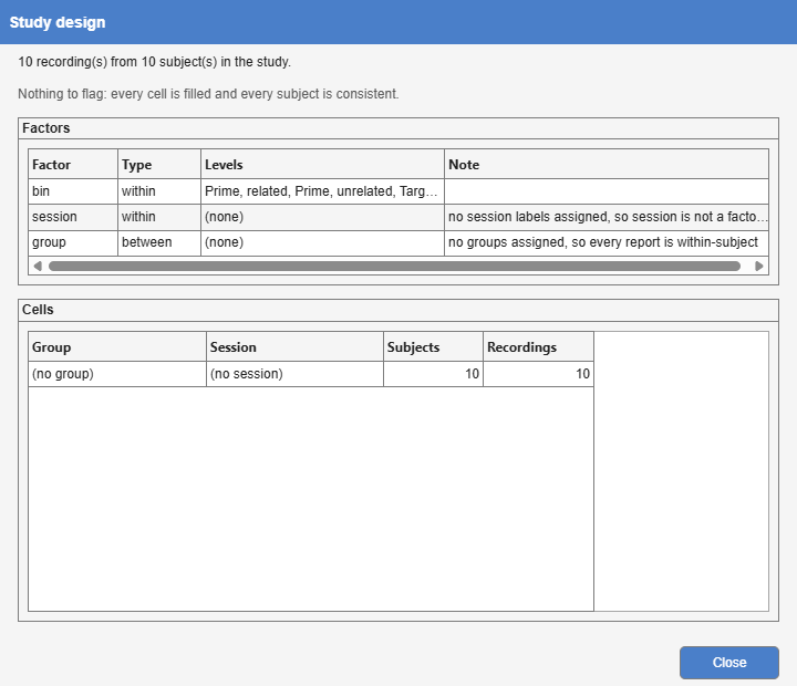
Alakazam > Design > Show Design (Figure 6.2) shows the design as the statistics will read it: the number of recordings and people, each factor with its levels, and a table of cells with the subjects in each. Above them it lists what is wrong, before any statistic is run: an empty cell, markedly unbalanced cells, a person with recordings in more than one group or with a group on only some of them, two recordings of one person in the same session, and subjects left without a group once groups are in use.
Figure 6.2: Show Design for the ten N400 recordings: one within-subjects factor (bin), no sessions and no groups, and one cell with every subject in it.
7 Reference: preprocessing
This chapter and the four after it describe every transformation, one section each, in a fixed order: what the step does and on what grounds, its options with their defaults, the dialog, a result where the result has a view of its own, and notes on its limits. Each section opens with a line giving the ribbon path, the formats it accepts and returns, and its internal name, which is the name a template or an exported script uses.
Conventions. Where EEGLAB or FieldTrip has a rule for an operation, Alakazam follows it, so that its numbers can be set beside theirs. A time window given in ms takes the nearest sample at each end, the earlier one when an end lies exactly halfway between two, and an end beyond the epoch takes the epoch’s own first or last sample, as FieldTrip selects a latency range; a window lying wholly outside the epoch is refused rather than replaced by the whole epoch. The exceptions follow the toolbox that does the same job: a time-frequency baseline takes the samples inside its window, as ft_freqbaseline and newtimef do, and so does Deconvolve’s baseline, as Unfold’s does. Rejected samples are left out of every mean and fit. Each section ends with Toolbox or own code: the toolbox that does the same job, and how Alakazam’s result is held to it.
The transformations of Tools > 1. Preprocessing are described here in the order in which they are usually applied rather than in the ribbon’s alphabetical order: first the channels and events, then the signal, then derived quantities, and last the two steps that work on epochs and averages.
7.1 ChannelEditor
Tools > 1. Preprocessing > ChannelEditor · any format → the same · ChannelEditor
Edits the channel labels, types and positions. Only the channel description changes; the data are untouched. This is what scalp maps, interpolation, ICA and the source estimates depend on, so it is the step to reach for when a recording arrives with the wrong labels, with no positions, or with a montage that is not the 10-20 system.
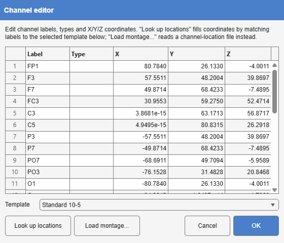
Figure 7.1: ChannelEditor: one row per channel with its label, type and Cartesian coordinates. Look up locations fills the coordinates by label from the chosen template.
Table 7.1: ChannelEditor’s controls.
Control
Effect
Table
Edit a channel’s Label, Type and X, Y, Z directly.
Template
The electrode template Look up locations reads: the standard 10-5 positions (Oostenveld and Praamstra 2001), or any montage file placed in src/Electrodes (an equidistant cap is included).
Look up locations
Fill every channel’s coordinates from the template, matching by label.
Load montage
Read positions from a channel-location file instead.
The edited channel description is stored, and on replay it is merged onto the other recording by label, so a correction made on one subject applies to every subject with the same channels.
7.2 EventEditor
Tools > 1. Preprocessing > EventEditor · continuous or epoched → the same · EventEditor
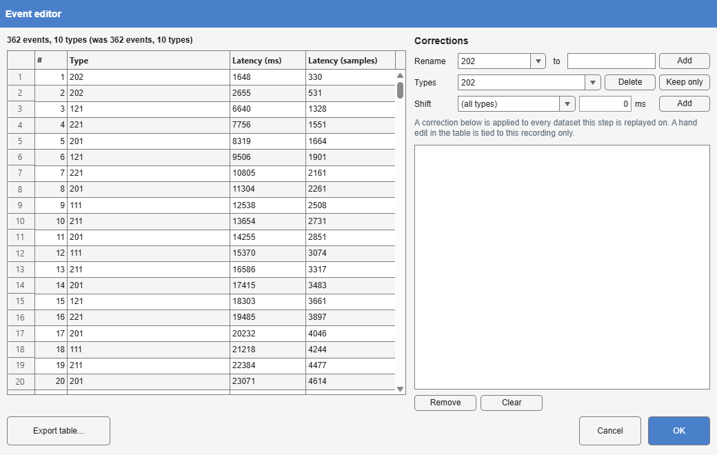
Corrects the event table: renames codes, removes the codes that are not stimuli, shifts latencies to correct a known delay, and fixes single events by hand. Doing this inside the tree, rather than in another program before import, keeps the correction in the record of the analysis and in an exported script.
Figure 7.2: EventEditor: the event table on the left, the list of corrections on the right. A correction in the list replays on every dataset; a hand edit in the table belongs to this recording.
Table 7.2: EventEditor’s corrections, applied in the order listed.
Correction
Effect
Renamecodetocode
Every event of one type becomes another.
Types > Delete
Remove every event of the chosen types.
Types > Keep only
Remove every event not of the chosen types.
Shifttypes by nms
Move the chosen events (or all) in time.
a cell of the table
Change one event’s type or latency.
What is stored is the list of operations, not the resulting table. Replayed onto another recording, “rename 112 to 121, then shift every 121 by -16 ms” applies the same correction to that recording’s own events, which is what a trigger fault (a property of the recording set-up) calls for. A shift is stored in milliseconds and converted with each recording’s own sampling rate. A hand edit is stored with the event’s original type and latency, and is applied on replay only to an event that still matches them.
Export table writes the event table to a file.
Not recalculable: the dialog opens on the dataset’s own events.
Toolbox or own code. EEGLAB’s pop_editeventvals edits events too, but an edit made there is not a step that Recalculate or Apply to All can replay; here every change is.
7.3 Photodiode
Tools > 1. Preprocessing > Photodiode · continuous → the same · Photodiode
A photodiode taped over a patch that changes with the stimulus records when the display actually changed. This step reads that channel and does one of two things: Measure (the default) pairs each light onset with the trigger that preceded it and reports the delay, changing nothing; Events adds the onsets to the event table, as EEGLAB’s pop_chanevent does, each named after its trigger with a suffix.
Measuring is the more useful of the two. A display adds a delay between the trigger and the change on the screen, typically of one or more frames, which shifts every latency in the study by the same amount, and only a photodiode can tell how large it is. The median delay is the value to correct by, with EventEditor’s latency shift (Section 7.2), since a dropped frame moves the mean but hardly the median. The report gives the number of pairs, the median, interquartile range and range of the delay, for all triggers and per trigger code.
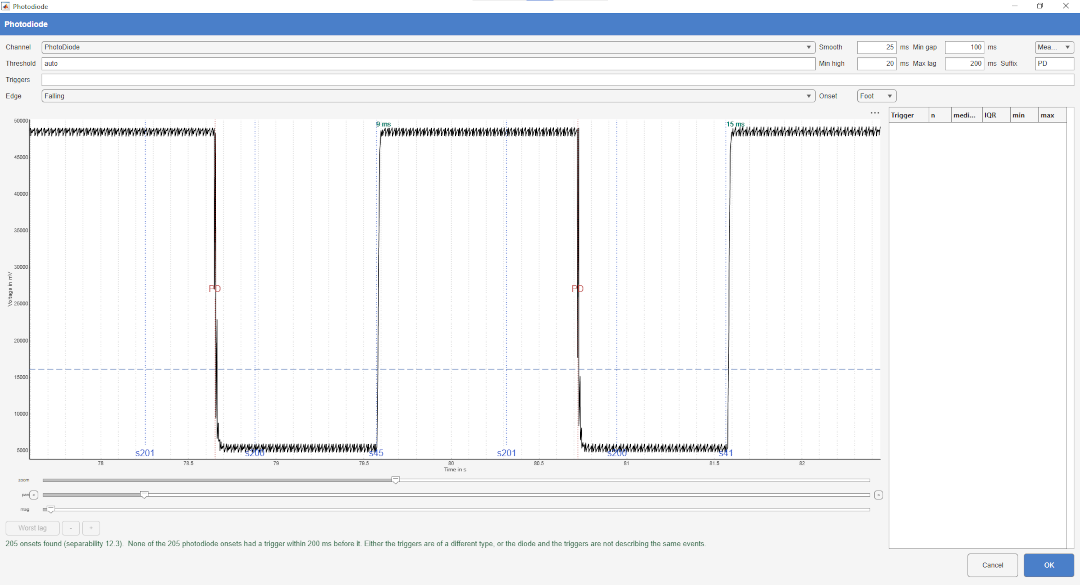
Figure 7.3: Photodiode on a recording with a diode patch, where light onset is a falling edge. The step found 205 onsets (separability 12.3) and marks them PD; none had a trigger in the 200 ms before it, and the step says so under the plot, leaving the delay table on the right empty.
7.3.1 Detecting onsets
Finding a step in a diode signal is easy; not finding one where there is none is the difficult part. A diode channel with no patch still swings at the mains frequency, and a plain threshold turns that into fifty onsets a second. Detection therefore has three stages:
The signal is smoothed with a moving average (25 ms by default), long enough to remove 50 and 60 Hz flicker while leaving a sustained change of level nearly intact.
The smoothed signal is tested for two states: split at the midpoint of its range, the distance between the two halves’ means, divided by the sum of their standard deviations, must be at least 3. A signal without patches is unimodal and fails the test, and the step then says so rather than reporting onsets. A threshold set by hand overrides the test.
Onsets are the crossings of a level a quarter of the way up the range, kept when the high state lasts at least Min high and the onset is at least Min gap after the previous one. Each is paired with the last trigger (of the listed codes, or any) within Max lag before it, or up to 5 ms after it, for a trigger sent at the moment of the display change rather than before it.
Table 7.3: Photodiode’s options.
Option
Default
Meaning
Channel
The photodiode channel.
Threshold
auto
The detection level; a number overrides the automatic level and the two-state test.
Triggers
all
The event codes an onset may be paired with.
Edge
Rising
Whether light onset is a rising or a falling edge on this rig.
Onset
Foot
Time the onset at the foot of the edge, or at half height.
Smooth
25 ms
The moving-average window.
Min high
20 ms
How long the high state must last.
Min gap
100 ms
The least time between two onsets.
Max lag
200 ms
How far before an onset its trigger may be.
Measure / Events
Measure
Report the delay, or add the onsets as events.
Suffix
PD
Appended to the trigger’s code to name an added onset event.
Not recalculable: the dialog opens on the dataset’s own signal.
Toolbox or own code. EEGLAB’s pop_chanevent turns a channel’s threshold crossings into events. Finding onsets at the foot or at half height, pairing each with the trigger that caused it, and measuring the delay and its spread have no toolbox equivalent, so they are Alakazam’s.
Joins the EyeLink recording of the same session onto the EEG, using EYE-EEG (Dimigen et al. 2011): the tracker’s clock is aligned with the EEG’s through the triggers both received, its gaze and pupil signals are added as channels of type EYE (which nothing treats as scalp EEG), and its saccades, fixations and blinks are added as events. Those events can then be binned like any other (fixation-related potentials) and modelled as covariates in deconvolution (Chapter 17).
The eye-tracking file is found by name: subject1.set goes with subject1.asc beside it, which is what lets one set of options be replayed on every subject. When only an .edf is present and SR Research’s edf2asc is installed, it is converted first.
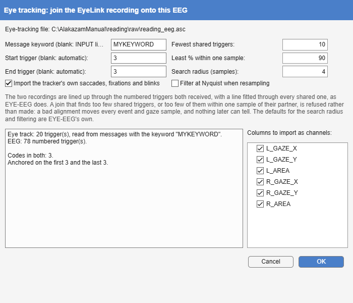
Figure 7.4: Eye tracking on EYE-EEG’s reading example: the triggers found in the tracker’s messages and in the EEG, the codes in both, and the columns to import.
Table 7.4: Eye tracking’s options.
Option
Default
Meaning
Message keyword
blank
The keyword of the EyeLink messages that carry the triggers (MYKEYWORD 123); blank reads the parallel-port input lines instead.
Start trigger, End trigger
automatic
The codes the alignment is anchored on (the first of the one, the last of the other); automatic takes the first and last code both recordings share.
Import the tracker’s own saccades, fixations and blinks
on
Add them as events.
Filter at Nyquist when resampling
off
EYE-EEG’s own option, and its default.
Fewest shared triggers
10
Refuse a join with fewer.
Least % within one sample
90
Refuse a join in which fewer of the shared triggers end up within one sample of their partner.
Search radius
4 samples
How far either side of an EEG trigger to look for its partner (EYE-EEG’s default).
Columns to import
all
The tracker’s columns to add as channels, by name.
A poor synchronisation is silent: every event lands a little away from the EEG it belongs to, and nothing downstream can tell. The join is therefore checked. EYE-EEG returns the dataset unchanged when it finds no shared triggers, and that is refused; its record of how far each shared trigger landed from its partner is summarised and refused below the two limits above; and the summary is kept, so that the data-quality report states the synchronisation for every subject (Chapter 15).
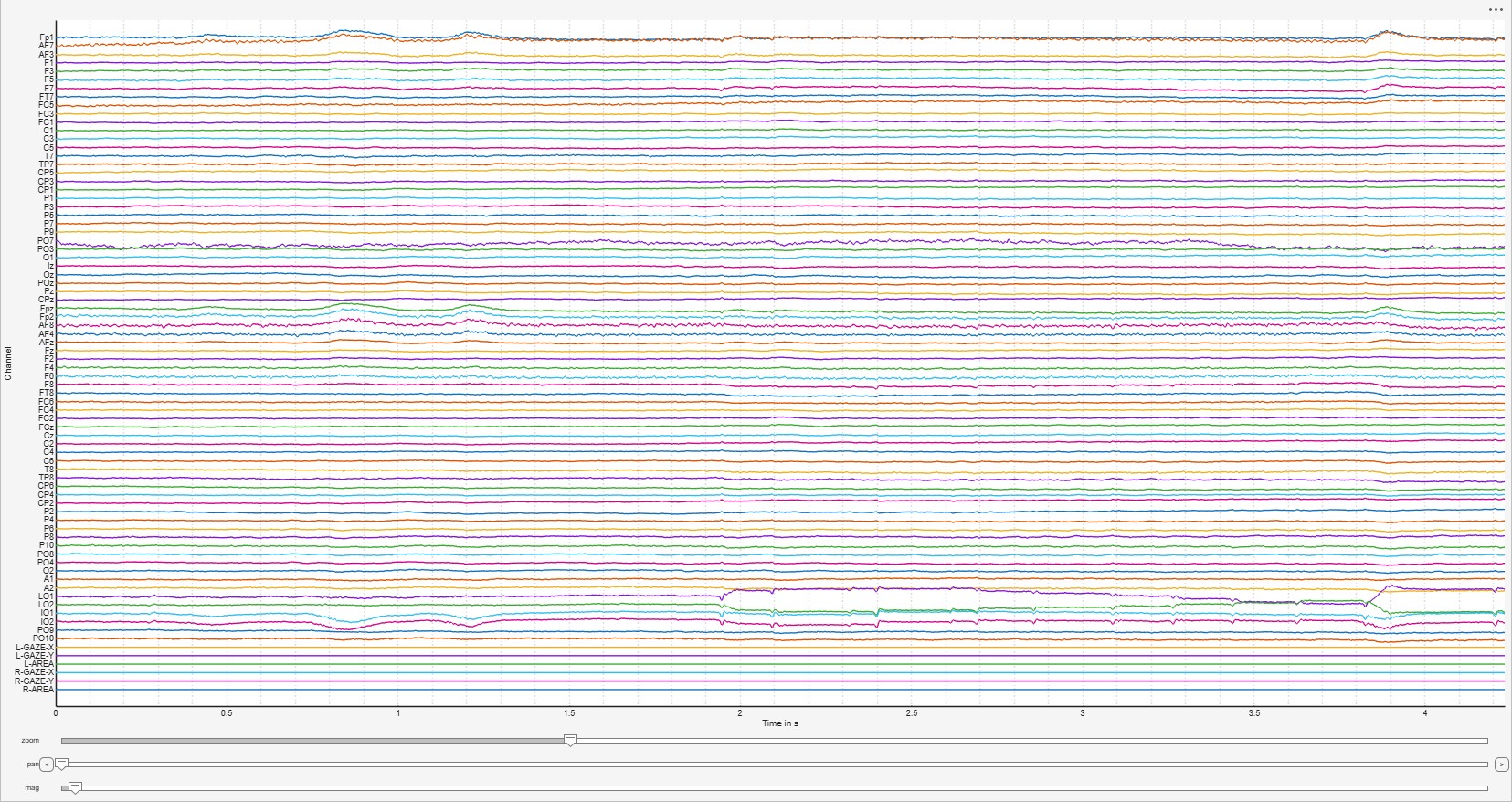
Figure 7.5: The reading example after the join: the gaze and pupil channels (L-GAZE-X to R-AREA) below the EEG.
Changes the sampling rate with EEGLAB’s pop_resample, which applies an anti-aliasing filter before decimating. Event latencies are rescaled with the data. Resampling is refused on epoched data: it belongs before segmentation, where every later step inherits the new rate.
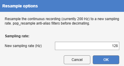
Figure 7.6: Resample. The field is prefilled with 256 Hz for faster recordings, and half the current rate otherwise.
Table 7.5: Resample’s option.
Option
Default
Meaning
New sampling rate
256 Hz, or half the current rate if that is lower
The new rate.
7.6 Filter
Tools > 1. Preprocessing > Filter · any time-domain format → the same · Filter
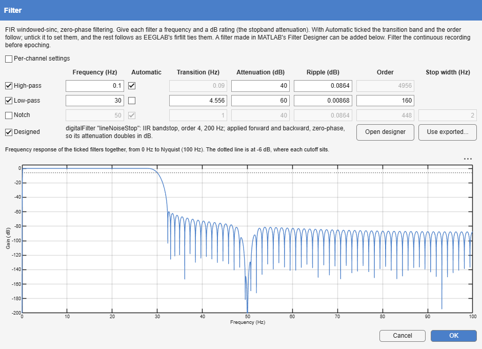
High-pass, low-pass and notch filtering with a zero-phase, linear-phase FIR filter: a windowed sinc with a Kaiser window, designed and applied by EEGLAB’s firfilt plugin (Widmann et al. 2015). Each filter is specified by a frequency and an attenuation; by default the order, the transition band and the window follow from them, and they can also be set (Section 7.6.2). The filter is applied with its group delay compensated, so it shifts no latency, and it does not filter across the boundaries of a discontinuous recording. A filter made in MATLAB’s Filter Designer app can be added as a fourth (Section 7.6.3).
Figure 7.7: Filter at 200 Hz: an automatic 0.1 Hz high-pass, a 30 Hz low-pass with its order set by hand (160, which at 60 dB gives a 4.56 Hz transition band), and a line-noise band-stop from the Filter Designer, applied forward and backward. The plot is their response together.
Table 7.6: Filter’s options.
Option
Default
Meaning
High-pass
off; 0.1 Hz, 40 dB
Remove frequencies below the cutoff.
Low-pass
off; 30 Hz, 40 dB
Remove frequencies above the cutoff.
Notch
off; 50 Hz, 40 dB
Remove a narrow band around the frequency (line noise).
Automatic
on
The transition band and the order follow from the frequency and the attenuation; unticked, they can be set.
Transition, Order
automatic
The transition band in Hz, and the filter order (the kernel has one tap more); each follows from the other.
Attenuation, Ripple
40 dB; 0.0864 dB
The stopband attenuation and the passband ripple: one deviation in two units.
Stop width
2 Hz
The notch’s stop band.
Designed
off
A filter made in MATLAB’s Filter Designer, applied after the other three.
Per-channel settings
off
Give each channel its own three filters, designed automatically; channels are matched by label on replay.
7.6.1 The design
The cutoff is the frequency at which the response is -6 dB, the centre of the transition band, which is how firfilt defines it (Widmann et al. 2015). The transition band is chosen from the cutoff f:
high-pass: 0.25f, but at least 1 Hz, and at most 0.9f;
low-pass: 0.25f, but at least 2 Hz, and at most 90% of the distance to the Nyquist frequency;
notch: a stop band of f ± 1 Hz, with 1 Hz transitions.
The ripple follows from the attenuation A: the stopband deviation is 10-A/20, and the Kaiser window’s order and are computed from it and the transition band. Table 7.7 shows what that means at 250 Hz and 40 dB.
Table 7.7: The filters Alakazam designs at 250 Hz and 40 dB stopband attenuation.
Filter
Transition band
Pass from
Stop at
Order
Length
high-pass 0.05 Hz
0.045 Hz
0.073 Hz
0.028 Hz
12 384
49.5 s
high-pass 0.1 Hz
0.09 Hz
0.145 Hz
0.055 Hz
6 194
24.8 s
high-pass 0.5 Hz
0.45 Hz
0.725 Hz
0.275 Hz
1 240
5.0 s
high-pass 1 Hz
0.9 Hz
1.45 Hz
0.55 Hz
622
2.5 s
low-pass 20 Hz
5 Hz
17.5 Hz
22.5 Hz
114
0.46 s
low-pass 30 Hz
7.5 Hz
26.25 Hz
33.75 Hz
76
0.31 s
notch 50 Hz
1 Hz
below 48.5, above 51.5 Hz
49.5 to 50.5 Hz
560
2.2 s
Two consequences follow. First, a low high-pass cutoff needs a very long filter: at 0.1 Hz, 25 seconds. Filter the continuous recording, before epoching; on data shorter than the filter, the step refuses and says so. Second, for high-pass cutoffs below about 1 Hz the transition band is 90% of the cutoff, so the passband begins well above the nominal frequency.
7.6.2 Setting the design yourself
Every filter shows its whole design: the transition band, the attenuation, the passband ripple and the order, and for the notch the width of its stop band. With Automatic ticked the transition band and the order are worked out as above and shown greyed. Untick it and they can be entered, and the rest follows as EEGLAB’s firfilt ties them: a Kaiser-windowed sinc has one deviation, 10-A/20, in its passband and its stopband alike, so the attenuation and the ripple are the same quantity in two units, and changing either changes the other. Entering a transition band, an attenuation or a ripple gives the order it needs (firwsord); entering an order gives the transition band it implies (invfirwsord), the attenuation kept. The order is always even, rounded up, since firws needs a type I filter. A shorter filter with a wider transition band, or a longer one with a steeper band, is the trade to make here; the plot below the filters shows the result.
7.6.3 A filter from the Filter Designer
MATLAB’s Filter Designer app designs filters of every kind: equiripple and least-squares FIRs, Butterworth, Chebyshev and elliptic IIRs, band-passes and band-stops. Open designer starts it. Design the filter in Hz for the data’s own sample rate, or in normalised frequency, then export it to the MATLAB workspace as a Digital Filter Object (or save it in a MAT-file), and press Use exported…, which lists the filters it finds and refuses one designed in Hz for another sample rate. Its coefficients are kept in the step’s options, so replaying it, a template and Apply to All need neither the app nor MATLAB’s workspace.
A filter designed in normalised frequency has no sample rate of its own: its band edges are fractions of the Nyquist frequency, and its coefficients are the same at any rate. It is read at the rate of the data it is chosen for, so on data sampled at 500 Hz a normalised frequency of 0.2 lies at 50 Hz, and the picker says where 1 lies. That rate is then kept as the filter’s own: replayed onto data sampled at another rate, it is refused like a filter designed in Hz, rather than having its band edges move with the rate.
The designed filter is applied after the other three, to every channel, in either mode. A linear-phase FIR of odd length is applied once, with its group delay compensated, like the filters above. Anything else, an IIR in particular, is applied forward and backward (filtfilt), zero-phase, as EEGLAB’s IIR filtering and FieldTrip’s default two-pass filtering apply one; its magnitude response is then squared, so its attenuation and its passband ripple both double in dB, and the plot shows the squared response, the one the data get. Each epoch, and each stretch of a continuous recording between boundaries, is filtered on its own, and so is each stretch between rejected samples, so that a rejected stretch does not spread through an IIR filter’s unending response; a stretch shorter than three times the filter’s order is left rejected, and the count is recorded.
7.6.4 Choosing the cutoffs
High-pass filtering is the step most capable of creating effects that are not in the data: a cutoff that is too high attenuates and distorts slow components and can produce deflections of opposite polarity before and after them (Tanner et al. 2015; Acunzo et al. 2012). A high-pass of about 0.1 Hz and, where one is wanted, a low-pass of about 30 Hz are the usual starting point for cognitive ERPs (Luck 2022). Zhang et al. (2024a) give a principled way to choose cutoffs for a given component and measure, trading the standardised measurement error against waveform distortion, and Zhang et al. (2024b) apply it to the seven ERP CORE components; their recommendations are the best current basis for a choice. Peak measures are more sensitive to high-frequency noise than mean amplitudes, and so benefit more from a low-pass. A notch filter is rarely needed after a 30 Hz low-pass.
Every filter also spreads a brief event over the length of its impulse response, and its ringing can pass for an oscillation. A methods section should therefore describe each filter in enough detail to reproduce it, ideally with a plot of its impulse or step response (Cheveigné and Nelken 2019); the type, cutoff, transition band and order in Table 7.7 are the details to give, and the step records the filters it applied in the result, with the whole design of each one in the panel. Under the filters, the dialog plots the frequency response of the ticked ones together, a designed filter included: the gain in dB from 0 Hz to the Nyquist frequency, with a dotted line at -6 dB, where each cutoff sits, and the axis reaching 20 dB below the deepest attenuation ticked, or, when a designed filter is ticked, 20 dB below the curve’s lowest point, down to -200 dB at most. It shows which frequencies pass, how steep each transition band is, and how far the stop bands reach; zoom in on a transition band with the plot’s toolbar to read it off. The plot is redrawn whenever a setting changes, and is not shown in per-channel mode. It is computed from the same kernels and coefficients the step applies, so it is the response of the filtering that is done.
Toolbox or own code. The design and the filtering are EEGLAB’s firfilt (firws, firwsord, invfirwsord, kaiserbeta, firfilt), and a designed filter is MATLAB’s (the Filter Designer’s digitalFilter, applied with filtfilt). What is Alakazam’s is the automatic choice of transition band, the dialog, and splitting the data where it must not be filtered across.
7.7 DC-Detrend
Tools > 1. Preprocessing > DC-Detrend · continuous or epoched → the same · DCDetrend
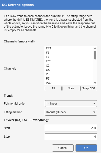
Removes a slow drift from each channel by fitting a low-order polynomial and subtracting it: per trial on epoched data, over the whole recording on continuous data. Order 0 removes the mean, order 1 a linear drift and order 2 a slow curvature, such as an electrode settling.
Figure 7.8: DC-Detrend, fitting a robust linear trend on the prestimulus interval only.
Table 7.8: DC-Detrend’s options.
Option
Default
Meaning
Channels
all
The channels to detrend.
Polynomial order
1 (linear)
0 (mean), 1 (linear) or 2 (quadratic).
Fitting method
Least squares
Or Robust (Huber).
Fit over start, stop
0 to 0 (everything)
The interval, in ms, over which the trend is estimated. It is always subtracted from the whole epoch.
The usual two-interval detrend (BrainVision Analyzer’s, for instance) runs a line through the means of a start and an end interval. This one differs in four respects:
It fits every sample in the fitting range, so one blink in the end interval no longer tilts the whole trend.
The fitting range and the subtraction range are separate. Fitting across the evoked response lets the response pull on the trend, so that the drift estimate absorbs part of the signal being measured. Fitting on the prestimulus interval, perhaps with a late tail, and extrapolating across the response avoids that.
A robust fit is offered: MATLAB’s robustfit with Huber’s weights (Huber 1964) (tuning constant 1.345), iterated to convergence, so that a large transient counts like a moderate one.
Rejected samples are left out of the fit and stay rejected. A channel with too few samples left to determine the fit is left untouched, and the count is reported.
Toolbox or own code. Both fits are MATLAB’s: least squares is polyfit, centred and scaled, on the samples of the fitting range that were not rejected, and the robust fit is robustfit. FieldTrip’s ft_preproc_polyremoval does the same least-squares fit, and on an epoch DC-Detrend matches it in the test suite; as FieldTrip calls it, though, it fits the raw sample index and loses an order-2 trend on a long continuous recording. MATLAB’s detrend fits over every sample it is given, and over the whole epoch DC-Detrend matches it too. The fitting range takes the nearest sample at each end, as above.
7.8 ReRef
Tools > 1. Preprocessing > ReRef · any time-domain format → the same · ReRef
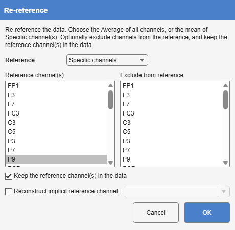
Re-references the data to the average of all channels, or to the mean of chosen channels, with EEGLAB’s pop_reref.
Figure 7.9: ReRef, re-referencing the ERP CORE N400 recording to the average of the mastoid-adjacent sites P9 and P10.
Table 7.9: ReRef’s options.
Option
Default
Meaning
Reference
Average
Average of all channels, or Specific channels.
Reference channel(s)
For specific channels: the channels whose mean is the new reference.
Exclude from reference
none
Channels left out of the reference and left unchanged (an EOG or a photodiode channel).
Keep the reference channel(s) in the data
off
Keep the reference channels, which are flat zero for a single reference and not for a mean of several.
Reconstruct implicit reference channel
off
Add back the channel the data were recorded against (below).
Channels are stored by label, so a stored reference replays on recordings whose channels differ in order.
The implicit reference. Many amplifiers record against one active electrode, often a mastoid or Cz, whose own signal is not saved because it is zero relative to itself. Re-referencing recovers it. Alakazam adds the channel back as a flat zero before re-referencing, as EEGLAB advises; if w is the waveform then subtracted from every channel, the old reference, which read zero, reads -w. The channel is inserted next to its nearest neighbour on the 10-5 template.
With an average reference, the reconstructed channel is part of the average: 32 recorded channels and the reference are averaged as 33 sites, and the channels sum to zero, as an average reference should. Channels excluded from the reference stay out of the average, and the reconstructed channel stays in it.
The choice of reference changes the shape of every waveform and map, and should follow the literature on the component studied, so that results can be compared (Luck 2022; Kappenman et al. 2021). An average reference assumes dense and even coverage of the head, which a 32-channel cap only approximates (Dien 1998).
7.9 Interpolate
Tools > 1. Preprocessing > Interpolate · continuous or epoched → the same · Interpolate
Rebuilds bad channels from the good channels around them, over the whole recording, with EEGLAB’s pop_interp. The number of channels does not change. For channels that are bad in some trials only, use the interpolate action of ArtefactDetect or ManualReject instead (Chapter 8).
Figure 7.10: Interpolate: the method, and the channels to rebuild.
Table 7.10: Interpolate’s options.
Option
Default
Meaning
Method
Spherical spline
Spherical spline(Perrin et al. 1989), Inverse distance, or EEGLAB’s spacetime method.
Channels to interpolate
none
The bad channels, with All and None to start from. Stored by label; OK asks for at least one.
Interpolation needs electrode positions (Section 6.1). An interpolated channel carries no information of its own, which reduces the rank of the data by one per channel: take this into account before ICA, and do not count an interpolated channel as an independent observation in a statistical test.
7.10 SelectData
Tools > 1. Preprocessing > SelectData · continuous or epoched → the same · SelectData
Keeps or removes channels, a time range, a range of samples, or trials, with EEGLAB’s pop_select. Each of the four can be set to Keep, Remove, or left off.
Figure 7.11: SelectData: channels from a list, time in seconds, points in samples, and trials by index.
Table 7.11: SelectData’s options.
Option
Default
Meaning
Channels
off
Keep or remove the chosen channels. Stored by label.
Time (s)
off
Keep or remove a time range, in seconds.
Points (samples)
off
Keep or remove a range of samples.
Trials (indices)
off
Keep or remove trials, written as MATLAB indices: 1:10, 15.
Selecting trials by index is tied to one recording’s trial order; to select trials by condition, use bins (Section 9.1).
7.11 Derive Channels
Tools > 1. Preprocessing > Derive Channels · any time-domain format → the same · DeriveChannels
Adds channels computed from existing ones, one let statement per line:
let LRP      = C3 - C4
let midline  = (Fz + Cz + Pz) / 3
let RMSfront = sqrt((Fz*Fz + Cz*Cz) / 2)
The grammar is small and is parsed, never evaluated as MATLAB: + - * / on channels and numbers, unary minus, parentheses, abs() and sqrt(), and % for a comment. The arithmetic is elementwise, so the step runs on continuous, epoched and averaged data alike. The block is checked when OK is pressed, against this dataset’s own channels and by the same parser the step runs, so a typo, an unknown channel or a name used twice is reported in the dialog rather than after the node exists.
Figure 7.12: Derive Channels on the ERP CORE LRP epochs, adding C34 = C4 - C3, the lateral motor pair; C4 is contralateral to a left-hand response.
Channel arithmetic and bin arithmetic are different operations, as in ERPLAB: a bin says which events go into an average (bin 3 = bin 1 - bin 2, in DefineBins), a derived channel says how to combine the channels of each of them. A derived channel has type derived and no scalp position: it is drawn in the waveform view and carried into grand averages, but left out of scalp maps.
Derived on an average, a channel has no confidence band and no aSME. Its standard error depends on how the channels it is computed from vary together over trials, which the average no longer holds, so it is left unknown rather than guessed. Derive it on the epochs instead, before Average, and Average gives it both, computed from its own trials as for any other channel.
Figure 7.13: The derived channel C34 in the response-locked LRP average: before a left-hand response (blue) C4 turns negative relative to C3, before a right-hand response (red) positive, and the LRP bin (teal), half their difference, is the contralateral-minus-ipsilateral negativity.
ERP Measure has a field for let statements too (Section 10.1). Each of the two replaces every derived channel when it runs, which is what makes a recalculation or a replay idempotent, so use one place or the other: derive here and leave Measure’s field empty.
Toolbox or own code. ERPLAB’s pop_eegchanoperator does channel arithmetic too, but ERPLAB is not one of the toolboxes Alakazam installs, and its formulas are not steps that Recalculate can replay. The arithmetic itself is MATLAB’s.
7.12 Rectify
Tools > 1. Preprocessing > Rectify · any time-domain format → the same · Rectify
Replaces the chosen channels with their magnitude or their square: the rectification step of an EMG-envelope analysis (rectify, smooth, measure).
Figure 7.14: Rectify: the channels, and the mode.
Table 7.12: Rectify’s options.
Option
Default
Meaning
Channels
The channels to rectify, with All, None and Scalp EEG (every channel that is not a known peripheral); required.
Mode
Full wave
Full wave (|x|), Half wave (negative values set to zero) or Squared (x2, in µV2).
Rectification does not commute with averaging. Rectifying single trials and averaging them gives a positive envelope whose baseline sits above zero, because it accumulates the magnitude of the noise; rectifying an average measures only the magnitude of the evoked response. For the squared mode the two orders have names: the average of squares is total power, including activity that is not phase-locked, and the square of the average is evoked power. Both orders are legitimate, and the step records with the dataset which channels it rectified, which order applied and, for the squared mode, the change of unit; the data-quality report shows all three per subject (Section 15.4). Rejected samples stay rejected.
Toolbox or own code. The operation itself is MATLAB’s absolute value or square; what Rectify adds is that it is a recorded, replayable step on the channels you choose.
Subtracts from every trial and channel the mean of a baseline interval. Each end of the interval takes the nearest sample, the earlier one on an exact tie, as FieldTrip and ERPLAB take it; rejected samples inside it are left out of the mean, as FieldTrip leaves them out, and stay rejected; an interval wholly outside the epoch is refused.
Figure 7.15: Baseline: the interval, in ms relative to the time-locking event, and a preview of it shaded over every channel’s average, redrawn as the interval changes.
Table 7.13: Baseline’s options.
Option
Default
Meaning
Start
-100 ms
Start of the baseline interval.
Stop
0 ms
End of the baseline interval.
Baseline correction is linear and so commutes with averaging: correcting the trials and then averaging gives the same waveform as averaging and then correcting (Luck 2014b). It is applied to the trials here, so that threshold-based artefact detection, which follows it, tests amplitudes relative to the baseline. An interval of 100 to 200 ms before the event is usual; a longer interval reduces noise in the correction, provided nothing event-related falls within it (Luck 2022).
Toolbox or own code. The rule is FieldTrip’s (the baseline window of ft_preprocessing) and ERPLAB’s, and the result matches FieldTrip’s in the test suite; it is one mean and one subtraction, so it is written out rather than called. EEGLAB’s pop_rmbase takes the samples inside the interval instead, so where the ends fall between samples it can differ by a sample.
Produces the contralateral and ipsilateral waveforms of a lateralised component, the N2pc (Luck and Hillyard 1994; Eimer 1996) or the LRP (Coles 1989), collapsed across every pair of lateral electrodes at once. Each bin is marked by the side of its stimulus (or the hand that responded), and two bins are added:
where and are the averages of the left-side and right-side bins. Each side is averaged before the two are combined, so the sides weigh equally however many bins each has; with one bin a side this is ERPLAB’s expression.
Figure 7.16: Collapse Hemispheres on an ERP CORE N2pc average: the left-target and right-target bins marked by side, the difference bin ignored, and the electrode pairs found by geometry.
Table 7.14: Collapse Hemispheres’ options.
Option
Default
Meaning
Side of each bin
ignore
Left, Right, or ignore.
Pair electrodes by
auto
geometry (mirroring positions through the midline), labels (10-20 odd and even numbers, or an L/R letter), or auto, geometry when positions exist.
Name the new bins
Contra, Ipsi
The labels of the two added bins.
The collapsed waveform of each pair is written to both of its electrodes, so that the new bins have the same channels as the old ones: the Contra bin at PO7 and at PO8 is the same contralateral waveform, scalp maps still draw, and a measurement window defined on PO7 keeps working. Midline and unpaired electrodes carry the plain mean of the two sides. Standard errors are propagated as for any combination bin (Section 9.2).
Figure 7.17: The N2pc of one ERP CORE subject at PO7: the contralateral waveform (orange) runs more negative than the ipsilateral one (black) from about 200 to 300 ms.
The contra-minus-ipsi difference alone can also be had without side assignments, by combining Derive Channels (let C34 = C4 - C3) with a difference bin (bin 3 = 0.5 bin 1 - 0.5 bin 2), which agrees with ERPLAB to within 10-14 µV. What that route cannot give is contra and ipsi separately, or every pair at once.
Toolbox or own code. ERPLAB reaches the same waveforms by composing a channel operation and a bin operation, as in Luck’s BinOps_Contra(Luck 2022); Alakazam does it in one step, and agrees with ERPLAB’s result to 6.7e-15 µV.
8 Reference: artefact rejection and correction
The transformations of Tools > 2. Artifact Rejection / Reduction deal with signal that is not brain activity: blinks and eye movements, muscle, drifts, bad electrodes. They fall into two families. Rejection removes the contaminated data, by trial or by channel within a trial (ArtefactDetect, AutoReject, ManualReject). Correction estimates the contaminating signal and subtracts it, keeping the trial (AutoICA, ICA, AutoGEDAI, ASR). PREP, the third kind, prepares the continuous recording: it removes line noise, finds and interpolates bad channels, and chooses the reference.
Three of these are the standardised, citable pipelines of the field: PREP (Bigdely-Shamlo et al. 2015), ASR (Mullen et al. 2015; Chang et al. 2020) and autoreject (Jas et al. 2017). Each replaces a judgement made by eye (which channels are bad, which bursts are artefact, which threshold rejects a trial) with a rule applied the same way to every subject, and each records what it did, so the data-quality report can say what it cost (Chapter 15).
Correction keeps more trials, and so more power, but it changes the data in ways that are harder to verify, and for time-locked ERPs of good quality aggressive correction does not reliably improve the result (Delorme 2023). Rejection loses trials, but what remains is the recording as it was. A common and defensible pipeline corrects blinks with ICA, then rejects what remains above a threshold (Luck 2022). Whichever is used, the data-quality report shows its cost per subject and condition (Chapter 15).
Rejection in Alakazam is marking, not deleting: rejected samples are set to NaN, the trial keeps its place, and Average leaves the NaN values out. This keeps trial numbers stable across the pipeline, which is what lets per-trial measures and single-trial models relate a trial to its neighbours.
Table 8.1: ArtefactDetect’s detectors. Several can be ticked; a channel trips if any of them flags it.
Detector
Flags a channel of a trial when
Absolute threshold
any sample lies outside [Minimum, Maximum] µV.
Step function
in a moving Window, advanced by Window step, the means of the first and second halves differ by more than Threshold µV: the signature of a saccade or the onset of a blink.
Moving-window peak-to-peak
the range (maximum minus minimum) within a moving Window exceeds Threshold µV.
Sample-to-sample
the difference between two consecutive samples exceeds Threshold µV: a single-sample jump.
Flat line
the voltage stays within Range within µV, peak to peak, for at least For at least ms: a disconnected electrode, a saturated amplifier or a dropout.
Figure 8.1: ArtefactDetect: the detectors, their thresholds and windows, the test interval, the channels tested, and what is done with a hit.
Table 8.2: ArtefactDetect’s options.
Option
Default
Meaning
Detectors
Absolute threshold
One or more of the five.
Minimum, Maximum
-100, 100 µV
The absolute threshold’s limits.
Threshold
100 µV
The limit of the other three detectors.
Window, Window step
200, 50 ms
The moving window of the step and peak-to-peak detectors.
Range within, For at least
1 µV, 200 ms
The flat-line detector’s tolerance and duration.
Test start, stop
0 to 0 (whole epoch)
The interval tested, in ms.
Channels
All channels
All channels, or Scalp EEG only.
Reject
Whole epoch
What to do with a hit (below).
A detector’s own settings are greyed out while it is not ticked.
What happens to a hit is chosen separately from the detection:
Whole epoch rejects every channel of the trial: the standard ERP practice, and the default.
This channel only rejects the offending channel of that trial and keeps the others, so that a noisy electrode does not cost the whole trial.
Interpolate this channel rebuilds the offending channel of that trial from its neighbours with spherical splines (Perrin et al. 1989). A channel without a scalp position (an EOG channel) cannot be interpolated and is rejected instead.
The flat-line detector tests the range of the voltage itself, so an electrode stuck at +40 µV is as flat as one stuck at zero, and every start position is tested, so no flat stretch falls between two windows. One flat channel is not an artefact: the reference electrode, which ReRef keeps (or reconstructs) as a channel of zeros. A channel that is exactly zero throughout is recognised as the reference and not tested; a channel that is zero in only some epochs is a dropout and is flagged.
Channels to test decides which channels can trip a trial. All channels includes the EOG channels, which is what makes a blink on VEOG reject the trial it falls in, and for ERP work that is usually the point. Scalp EEG only leaves the peripheral channels untested, for when a threshold chosen for the scalp would be wrong for them.
Interpolation deserves caution. Unlike rejection, an interpolated channel looks like ordinary data, so Alakazam records which channel of which trial it rebuilt, and the data-quality report shows how much of each subject’s data is reconstructed rather than recorded. And a spatially broad artefact, such as a blink, is present on the neighbours too, so interpolating the worst channel copies the artefact rather than removing it: interpolation suits a single bad electrode, not a blink.
Figure 8.2: The epochs of the ERP CORE N400 recording at FP1 after ArtefactDetect, grouped by bin in recording order. Rejected trials are blank rows.
8.1.1 Which detector cost which trials
With several detectors ticked, knowing that a trial was rejected is not knowing why. ArtefactDetect records, per detector, the epochs it would have rejected on its own and the epochs only it caught. A node’s context menu Rejection breakdown shows them (Figure 8.3), here for the N400 epochs of Figure 8.2 tested with three detectors (±100 µV, a 100 µV step, and 100 µV peak-to-peak, both in a 200 ms window stepped by 50 ms, on all channels).
Figure 8.3: Rejection breakdown for three detectors: 93 of 231 epochs rejected in all, and per detector the epochs it would have rejected on its own, those no other detector caught, and the channel-epochs it flagged.
The per-detector counts overlap, since one blink trips several detectors, so they do not add up to the total. The “only this one” column is the number to read before switching a detector off or moving its threshold: here the step detector rejected 82 epochs, but none that the other two did not also reject, so switching it off would change nothing.
8.1.2 Choosing thresholds
Fixed thresholds of ±100 µV, or 100 µV peak-to-peak, are the usual starting point, but the right value depends on the recording and the subject, and Luck recommends choosing per subject from the data, by looking at which trials a threshold catches and which it misses (Luck 2022). The standardised measurement error gives an objective criterion: the threshold that minimises the SME of the score being analysed, which trades the noise removed against the trials lost (Luck et al. 2021). A rejection rate above about 25% of the trials in any condition is the conventional point at which a subject is excluded, and the data-quality report flags it. AutoReject, below, chooses a threshold per channel from the data itself.
Toolbox or own code. The detectors are ERPLAB’s, written in Alakazam because ERPLAB marks whole epochs, where Alakazam can reject or interpolate one channel of a trial and records each detector’s verdicts. On Luck’s data (Luck 2022) they flag the same 346 of 346 trials as ERPLAB’s absolute threshold, and 345 of 346 with the moving window, the one difference an artefact ERPLAB misses.
Learns the rejection thresholds from the data, by the local autoreject algorithm (Jas et al. 2017). A fixed threshold treats every channel alike, although a frontal channel near the eyes and an occipital one far from them differ in how much they vary; and it is chosen by eye. AutoReject instead chooses, for each scalp channel, the peak-to-peak threshold that the data support, and then decides, per epoch, whether to reject it or repair it:
A threshold per channel, by cross-validation. The epochs are split into ten blocks. For a candidate threshold, the epochs of nine blocks that stay under it are averaged, and the average is compared with the median of the tenth block, a robust stand-in for the clean response. A threshold that lets artefacts in pulls the average away from the median; one that throws good epochs away makes it noisy. The threshold with the smallest error over the ten blocks is the channel’s.
Bad channels per epoch. A channel is bad in an epoch when its peak-to-peak amplitude there exceeds its threshold.
Reject or repair. An epoch with too many bad channels is rejected. In the others, up to a set number of bad channels, the worst, are interpolated from the rest of the epoch. How many is too many (the consensus) and how many are interpolated are chosen by the same cross-validation.
Figure 8.4: AutoReject with its defaults: ten folds, and autoreject’s own candidates for the number of channels to interpolate.
Table 8.3: AutoReject’s options. The consensus is chosen from 0 to 1 in steps of 0.1, as in autoreject.
Option
Default
Meaning
Folds
10
The number of blocks the cross-validation uses.
Interpolate at most (candidates)
blank
The numbers of channels to consider interpolating per epoch; blank uses autoreject’s own, 1, 4 and 32 (at most one fewer than the channels).
Only the scalp channels with a position are tested and interpolated, each from the others; peripheral channels are left alone, as autoreject leaves everything but the EEG. Epochs already rejected are passed through and not counted. As everywhere in Alakazam, a rejected epoch is NaN on every channel, and the interpolated channel-epochs are recorded, so the data-quality report shows the share of the data that was rebuilt; its provenance section lists, per subject, the epochs rejected, the channel-epochs interpolated and the range of the learnt thresholds.
Figure 8.5: The epochs of the ERP CORE N400 recording at FP1 after AutoReject, grouped by bin in recording order. Rejected epochs are blank rows; in the others, the channels found bad were interpolated.
The folds are autoreject’s own, contiguous and not shuffled, so the result is deterministic and a replay reproduces it. Two details differ from the Python package, on purpose. Each threshold is the exact minimum of the cross-validation error over every candidate, where autoreject samples 50 of them by Bayesian optimisation. And each number of channels to interpolate is scored from the thresholded channels alone, where autoreject’s cross-validation carries one candidate’s interpolations into the next. Both are the algorithm as the paper states it.
Toolbox or own code. Autoreject exists only as a Python package, so it is implemented in Alakazam, with the differences described above; its repairs use EEGLAB’s interpolation.
The manual counterpart of ArtefactDetect: a browser that shows every channel of one trial at a time, in columns of at most 16 channels, where a click on a channel’s trace or label flags that channel of that trial. Prev and Next, or the left and right arrow keys, walk through the trials; flags persist while paging. Scale sets the amplitude gain for every trace, on top of one robust starting scale shared by all channels and trials, so that paging between trials remains a comparison by eye.
Figure 8.6: ManualReject on the ERP CORE MMN data: one trial’s channels in two columns, with the scope and the treatment of single channels at the bottom.
Table 8.4: ManualReject’s options.
Option
Default
Meaning
Reject
Whole epoch
Whole epoch: a flag rejects the trial. This channel only: it rejects that channel of that trial.
Single-channel treatment
NaN
For This channel only: leave the flagged cell rejected, or Interpolate it from its neighbours.
The flags are specific to this dataset’s trials, and a replay onto a dataset with a different number of trials is refused rather than applied to the wrong ones. Recalculating the node reopens the browser with the same flags, since recomputing its input leaves the trials where they were.
8.4 AutoICA
Tools > 2. Artifact Rejection / Reduction > AutoICA · continuous or epoched → the same · AutoEyeICA
Decomposes the data with independent component analysis (ICA), classifies the components with ICLabel (Pion-Tonachini et al. 2019), and subtracts every component whose probability of being an eye component exceeds a threshold. ICA separates the recording into maximally independent sources with fixed scalp maps (Jung et al. 2000); blinks and eye movements form a few components with a characteristic frontal map, and subtracting them removes the ocular signal from every channel while keeping the trials.
Figure 8.7: AutoICA: the ICLabel eye probability above which a component is removed.
Table 8.5: AutoICA’s option.
Option
Default
Meaning
Probability
0.8
Remove components whose ICLabel eye probability exceeds this.
The algorithm. FastICA (Hyvärinen and Oja 2000) is used when it is installed (it is offered on first use); otherwise EEGLAB’s ICA dialog opens, whose default is runica, extended Infomax (Bell and Sejnowski 1995). Classification uses ICLabel’s beta classifier. Only channels with a scalp position on the 10-5 template, and not typed as peripheral, are decomposed; EOG, ECG and other channels are set aside and put back unchanged.
Reproducibility. ICA starts from a random point, so two runs on the same data give slightly different components. The decomposition and the classification do not depend on the threshold, so they are kept with the node: changing the threshold with Recalculate re-prunes the components already found instead of decomposing again, and rerunning on unchanged data reuses the earlier decomposition. A new decomposition can be forced by setting Redecompose to true in the stored options.
Preparing the data. ICA finds better-separated components on data high-pass filtered at 1 to 2 Hz (Winkler et al. 2015), a cutoff too high for most ERP analyses (Section 7.6). One way to have both is to run AutoICA on a branch filtered at 1 Hz for inspection, and to compare the result with the same pruning on a 0.1 Hz branch. Interpolated channels and an average reference each reduce the rank of the data by one, and a decomposition cannot have more components than the rank.
Free viewing. With many eye movements, as in reading or visual search, ICA trained with the usual settings leaves ocular artefacts in the data, among them the spike potential at saccade onset. Correction improves greatly when the training data are high-pass filtered and the stretches around saccade onsets are heavily overweighted (Dimigen 2020). AutoICA does neither of these for you: it decomposes the data as they come.
8.5 ICA
Tools > 2. Artifact Rejection / Reduction > ICA · continuous or epoched → the same · RemoveComponents
The manual counterpart of AutoICA: a table of every component with the class ICLabel gave it and that class’s probability, followed by the probability of every class, and a preview of the selected component’s scalp map, the start of its time course, and its power spectrum. Tick the components to subtract. The dataset’s existing decomposition is used when it has one (after AutoICA, say); otherwise ICA is run first, as in AutoICA.
Figure 8.8: ICA on the ERP CORE MMN recording: each component’s ICLabel class and probabilities, sortable by any column, and a preview of the selected component.
The per-class probabilities are shown because a component labelled “Brain 53%” against a close runner-up is a different proposition from one labelled “Brain 99%”. Sorting by a class’s column brings all the eye or muscle components together. When dipole fitting is available, a Dipole RV column gives the share of the component’s scalp map that a single equivalent dipole cannot explain. Components of cortical origin tend to be close to dipolar (Delorme et al. 2012); the dialog treats a residual variance above about 15% as a sign that a component is not one compact cortical source, and “no fit” as a stronger sign still.
Not recalculable: component numbers belong to one decomposition, and a new decomposition numbers its components differently.
8.6 AutoGEDAI
Tools > 2. Artifact Rejection / Reduction > AutoGEDAI · continuous or epoched → the same · AutoGEDAI
Denoises with GEDAI (Ros et al. 2025), which separates brain signal from artefacts by a generalised eigenvalue decomposition of the data’s covariance against a reference covariance derived from a head model’s leadfield: activity whose spatial structure a cortical source could produce is kept, and the rest is removed, with the boundary between the two chosen automatically by GEDAI’s SENSAI criterion. It is broadband, so it addresses muscle and electrode noise as well as ocular artefacts, and it can be used instead of AutoICA or after it.
Figure 8.9: AutoGEDAI: the denoising strength, the leadfield, the epoch size, the low cut, the sliding window, and optional rejection of epochs and channels by their ENOVA.
Table 8.6: AutoGEDAI’s options, as GEDAI’s own dialog asks them. GEDAI’s other settings are left at its own defaults; a step saved before the epoch size and the sliding window were offered runs with their defaults, as it did then.
Option
Default
Meaning
Denoising strength
auto
auto; auto+ removes more noise at some cost to signal, auto- keeps more signal at some cost in noise.
Leadfield matrix
precomputed
GEDAI’s precomputed leadfield, matched by channel label, or interpolated to the montage.
Epoch size (wave cycles)
12
How long a stretch GEDAI judges at a time, in cycles of each wavelet band’s lowest frequency: 12 cycles are 1.5 s in a band starting at 8 Hz, and longer in slower bands.
Low-cut frequency
0.5 Hz
Wavelet bands below this frequency are removed, which high-pass filters the output.
Sliding window
Inf
Inf sets one threshold for the whole recording. A number of seconds lets the threshold follow noise that changes over the recording, recomputed in windows of that length.
Reject bad epochs, Epoch ENOVA threshold
no, 0.9
Reject GEDAI’s internal epochs whose share of variance explained as noise (ENOVA) exceeds the threshold.
Reject bad channels, Channel ENOVA threshold
no, 0.9
The same for channels, which GEDAI then interpolates back.
Use parallel processing
Honoured only when a GPU is present (below).
Three properties of the output are easy to miss:
It is average-referenced. GEDAI re-references the scalp channels to their average (in a form that does not reduce the rank of the data) before denoising, and returns them that way.
It is high-pass filtered at the low cut, by the removal of the wavelet bands below it.
Rejected epochs are marked, not cut. GEDAI removes a rejected stretch from the data; Alakazam puts it back as rejected (NaN) on every channel, so that the recording keeps its length and its events their latencies. Rejected channels are interpolated by GEDAI and keep their place.
Only channels in GEDAI’s 10-5 template are denoised; the others are set aside and put back unchanged. GEDAI’s diagnostics (the SENSAI score and the ENOVA per epoch and per channel) are kept with the result, and so is the GEDAI version that ran.
GEDAI is not bundled, and its licence (PolyForm Noncommercial 1.0.0) allows noncommercial research use only (Table 2.1). AutoGEDAI runs its newest release. The first run downloads it, after consent. After that, once in each MATLAB session, AutoGEDAI asks GitHub whether a newer release is out; if one is, it is installed beside the older ones, without asking again, and used from then on. Offline, or when the download fails, the newest installed release runs. A new release can change the result, so the version is recorded, and a step replayed later runs the release installed then, not necessarily the one it first ran with.
Its parallel processing on the CPU can silently corrupt the output when one of its frequency bands fails and is retried, so Alakazam uses parallel processing only on a GPU; the problem has been reported to its authors.
Runs the PREP pipeline (Bigdely-Shamlo et al. 2015), the standardised early stage of preprocessing that large EEG studies cite as one step. PREP removes line noise at the mains frequency and its harmonics, leaving the rest of the spectrum alone; then it estimates a robust average reference, the average of the channels that are not bad, where a channel is bad by extreme amplitude, poor correlation with the others, excess high-frequency noise, or poor prediction from its neighbours (RANSAC). Which channels look bad depends on the reference, and the reference depends on which channels are bad, so the two are estimated in turn until they agree. The bad channels are then interpolated and every channel is put on the robust reference.
Figure 8.10: PREP on the unreferenced ERP CORE N400 recording, with the line frequency set to 60 Hz, the mains frequency where it was recorded.
Table 8.7: PREP’s options, with PREP’s own defaults except the line frequency, which PREP sets to 60 Hz.
Option
Default
Meaning
Line frequency
50 Hz
The mains frequency; its harmonics below the Nyquist frequency are removed too. none skips the step.
Robust deviation
5
A channel whose robust z-score of amplitude exceeds this is bad.
High-frequency noise
5
The same for its noise above 50 Hz relative to its signal.
Minimum correlation
0.4
A channel correlating less than this with the others, in too many one-second windows, is bad.
Predict from neighbours
on
RANSAC: a channel its neighbours predict poorly is bad. Turn off for a small montage.
Ignore boundary events
off
PREP refuses a recording with discontinuities; ticking this runs across them.
The reference is estimated from, and bad channels are looked for among, the scalp channels with a position. EOG channels are cleaned of line noise and put on the same reference, so an eye channel stays comparable with the scalp, but they do not shape the reference and are not interpolated. Any other channel (ECG, a photodiode) is left as it was. PREP high-passes a copy of the data to decide which channels are bad; the data it returns keep their low frequencies, so Filter them as the analysis needs.
PREP’s full record stays with the result, and what a methods section needs (the channels interpolated, those still noisy after referencing, the line frequencies and the version) goes to the data-quality report. PREP is downloaded on first use, after consent (Table 2.1).
8.8 ASR
Tools > 2. Artifact Rejection / Reduction > ASR · continuous → continuous · ASR
Artifact Subspace Reconstruction, from EEGLAB’s clean_rawdata plugin (Mullen et al. 2015). It first finds scalp channels that are flat for too long or that their neighbours predict poorly, and interpolates them. Then it learns, from the cleanest stretches of the recording, what the scalp’s covariance normally looks like; wherever a sliding window’s variance exceeds that by more than the burst criterion along some direction, the offending components are reconstructed from the clean ones. Large, brief artefacts (movement, electrode pops, muscle bursts) are repaired, and the rest of the recording is untouched.
Figure 8.11: ASR with its defaults, on the filtered ERP CORE N400 recording.
Table 8.8: ASR’s options. The criterion defaults to 20, the value clean_rawdata’s own dialog proposes, within the 20 to 30 found to work on real EEG (Chang et al. 2020).
Option
Default
Meaning
Flat for longer than
5 s
A channel flat for longer than this is bad; 0 switches the check off.
Correlation below
0.8
A channel correlating less than this with its prediction from its neighbours, for more than half the recording, is bad; 0 switches it off.
Line noise above
4 SD
A channel with this much more line noise than the rest is bad; 0 switches it off.
Burst criterion
20 SD
How far a window may exceed the calibration before it is repaired. Lower is more aggressive.
Bursts are
Repaired
Repaired, or Rejected: every sample ASR would change is marked rejected instead.
Reject bad windows, Bad above
off, 0.25
After the repair, reject windows in which more than this fraction of the channels are still out of range.
ASR assumes data without slow drifts, so high-pass the recording first (Filter, about 0.5 to 1 Hz). clean_rawdata applies its own high-pass inside the same function; here it is left to Filter, so that each operation is a step of its own in the tree, and ASR warns when the recording still carries large offsets. The flagged channels are interpolated back in their own places, so the montage is unchanged. A rejected stretch is marked rejected (NaN) on every channel rather than cut out, so the recording keeps its length and its events their latencies; an epoch cut across it keeps NaN there, which Average leaves out sample by sample. Only scalp channels with a position calibrate ASR and are cleaned; the others are left as they were.
clean_rawdata ships with EEGLAB and is installed through EEGLAB’s plugin manager when it is missing. The data-quality report lists, per subject, the channels interpolated, the share of samples repaired and rejected, and the criterion used.
9 Reference: epoching and averaging
Tools > 3. Epoching and Averaging turns a continuous recording into event-related responses. DefineBins says which events belong to which condition and cuts epochs around them; Average averages each condition; and Deconvolve is the alternative to both when the responses to successive events overlap in time.
9.1 DefineBins
Tools > 3. Epoching and Averaging > DefineBins · continuous → epoched, or continuous with bin tags · DefineBins
Assigns events to bins with a small event-selection language, and cuts an epoch around every matched event. It replaces ERPLAB’s EventList and BINLISTER steps (Lopez-Calderon and Luck 2014). Each bin is one statement, a condition on the events of the recording; every event that meets it becomes a time-locking point (0 ms) of that bin.
Figure 9.1: DefineBins with the ERP CORE N400 bins: primes and targets by relatedness, a target counted only when a correct response follows within 200 to 1500 ms, and the N400 difference as a combination bin.
Table 9.1: DefineBins’ options.
Option
Default
Meaning
Epoch start, Epoch stop
The epoch around each matched event, in ms, when the script has no epoch line. With neither: tag the events with their bins and leave the data continuous.
script
The bin definitions, in the language below.
Save, Load
Write or read the script and the epoch together, as a .binscript file.
Import BDF
Translate an ERPLAB bin descriptor file into the language (below).
Syntax
Open the language reference.
The script is compiled when the dialog closes, and the compiled form, not the text, is what a replay evaluates on another recording’s events. Apart from comments (% or # to the end of the line), a script is a series of statements, each starting with bin, let or epoch; anything else before the first of them is an error rather than being dropped. Every error is reported with its line, a caret under the mistake and an explanation of how to fix it.
9.1.1 The bin language, in eleven steps
A bin is a number, a quoted label, and a condition. The simplest condition is an event code:
bin 1 "Targets" 112
Several codes are written with a pipe, or as a braced list; a quoted code may use the wildcards ? (one character) and * (any run). Matching is case-insensitive.
bin 1 "Targets or probes"   112|122
bin 2 "Any of five stimuli" {"s11" "s22" "s33" "s44" "s55"}
bin 3 "Any two-digit s"     "s??"
A relation constrains a neighbouring event:
Table 9.2: The relations of the bin language.
Relation
True when
next(code)
a following event of that code exists (the nearest one)
prev(code)
a preceding event of that code exists (the nearest one)
adjacent(code)
the very next event, whatever it is, has that code
any(code) within W
an event of that code lies inside window W
A window restricts a relation in time. Windows are signed (positive is after the event) and explicit about open and closed bounds:
bin 1 "Answered in time" 112 and next(118) within (200,1200] ms
within (200,1200] ms     % more than 200 and at most 1200 ms after
within [-1200,-200) ms   % before the event
within (0,300] samples   % in samples
within [-2,-2] events    % exactly two events back
The events unit counts positions in the event stream rather than elapsed time. In a strict stimulus, response, stimulus design, prev(112) within [-2,-2] events finds the stimulus of the previous trial whatever the interval was, where a time window wide enough to absorb variable reaction times could reach into the trial before.
Terms combine with and, or and not (in that order of precedence, not binding tightest), grouped with parentheses. Adjacent terms are joined by and even without the keyword, which reads well for exclusions:
bin 2 "Related, no answer" 112 and not next(118) within (0,2000] ms
bin 4 "Unrelated" "s??" not {"s11" "s22" "s33"} and next("S201") within (200,1200] ms
Reaction times come for free. When a bin matches through a forward relation, the delay to that neighbour is recorded as the trial’s reaction time, and rt within filters on it:
bin 1 "Fast" 112 and next(118) rt within (200,500] ms
bin 2 "Slow" 112 and next(118) rt within (500,1200] ms
The reaction time is the delay to the neighbour found by the first forward relation that contributed to the match; a backward relation such as prev(cue) never provides it. A match without one is dropped by rt within. The reaction time also becomes a sort key of the ERP image (Section 5.3).
The epoch is a statement of its own, shared by all bins, in the same interval notation as a window:
epoch [-200,800] ms
bin 1 "Targets" 112
Its unit is ms (the default) or samples, never events, and an epoch keeps both of its ends, so round and square brackets mean the same here. It may stand anywhere in the script, once. When the script has an epoch line, it wins over the Epoch start and Epoch stop fields, and the summary after the run says so if the fields held something else; this is what lets a script, a .binscript file or a template carry its own epoch.
Response-locking moves time zero to a neighbour with timelock, while membership is still decided by the condition:
bin 1 "Response-locked" 112 and next(118) timelock next(118)
Names.let names any piece of a condition, a set of codes or a whole relation, which is the way to write a relation once and use it in every bin:
let related  = {"s11" "s22" "s33" "s44" "s55"}
let answered = next("S201") within (200,1200] ms

bin 1 "Related"   related and answered
bin 2 "Unrelated" "s??" not related and answered
A name may use names defined before it, and a relation inside a name means exactly what it would mean written out where the name is used.
Difference bins are arithmetic on other bins’ averages, with integer or fractional coefficients:
bin 3 "N400 effect" = bin 2 - bin 1
bin 4 "Mean of two" = 0.5 bin 1 + 0.5 bin 2
They have no trials of their own. Average forms them from the averages of the bins they name, and their standard error from those bins’ standard errors (Section 9.2).
Interactions are combination bins of combination bins, nested to any depth, in any order of declaration:
bin 5 "Relatedness, expected"    = bin 2 - bin 1
bin 6 "Relatedness, unexpected"  = bin 4 - bin 3
bin 7 "Relatedness x Expectancy" = bin 6 - bin 5
A cycle, or a reference to a bin that does not exist, is an error when the script is compiled.
9.1.2 Codes and matching
Table 9.3: How codes are matched.
Written as
Matches
112
the markers 112, "112", S112 and S 112
"R201"
the marker R201; text must be quoted, since a bare word is a name
21-30
every code from 21 to 30, with or without the S prefix
"1??"
a pattern: wildcards work inside quotes only
A leading S before digits is dropped on both sides, so BrainVision’s S 12 and a plain 12 are the same code; a response marker keeps its R, since R 12 usually reuses the number of the stimulus it answers. Spaces inside a marker are ignored. A range is expanded to every code it covers, up to 1000 codes.
9.1.3 Importing ERPLAB bin descriptors
Import BDF reads a BINLISTER bin descriptor file and translates it: the time-locking event .{a;b} becomes the code set a|b, a preceding bracket {c}.{...} becomes prev(c), and a following bracket with a time condition .{...}{r:200<t<=800} becomes next(r) within (200,800] ms. What has no equivalent (write-back flags, flag conditions, open-ended times) is imported as far as it goes and marked with a % WARNING: line to finish by hand.
9.1.4 Grammar
script   : ( let | bin | epoch )+      (only comments before the first)
epoch    : epoch <window>             (ms or samples; at most once)
let      : let <name> = <expr>
bin      : bin <int> "<label>" [:] <expr> [timelock <relation>] [rt within <window>]
         | bin <int> "<label>" = <combo>
combo    : [coeff] bin <int> ( (+|-) [coeff] bin <int> )*
expr     : expr or expr | expr [and] expr | not expr | ( expr ) | <codes> | <relation>
relation : next(<codes>) [within <window>] | prev(<codes>) [within <window>]
         | adjacent(<codes>) [within <window>] | any(<codes>) within <window>
codes    : <code> ( | <code> )* | { <code> [,] <code> ... } | <name>
code     : <integer> | <integer>-<integer> | "<marker>"
window   : ( or [ <num> , <num> ) or ] [ms | samples | events]
comment  : % or # to the end of the line
9.1.5 The result
With an epoch, DefineBins returns an epoched dataset: one epoch per matched event, a trial in several bins stored once and listed in each. Without one, the data stay continuous and each event carries its bin membership, which is what Deconvolve fits against. The time to the next and to the previous event of every type is measured for each trial as it is cut, and becomes a sort key of the ERP image (Figure 3.2).
Toolbox or own code. DefineBins replaces ERPLAB’s EVENTLIST and BINLISTER; an ERPLAB bin descriptor file is translated into a bin script rather than run. On Luck’s N2pc data (Luck 2022) it puts 642 of 642 events in the same bins as BINLISTER, and its epochs are identical to ERPLAB’s.
9.2 Average
Tools > 3. Epoching and Averaging > Average · epoched → averaged · Average
Averages the trials of each bin, separately, giving one waveform per bin with its standard error; without bins it averages all trials. A trial in several bins contributes to each. Average has no options.
Figure 9.2: The N400 recording’s average at CPz: one waveform per bin with its ±n SE band, the trial counts in the legend, and each bin’s aSME on the right.
For each bin, channel and time point, with the kept trials:
the average is the mean over the trials that were not rejected;
the standard error is , with the standard deviation over the kept trials and their number there, so that a channel rejected in some trials only has the larger error it should have;
the analytic standardised measurement error (aSME) of the mean amplitude over the whole epoch is the standard deviation of the trials’ mean amplitudes divided by (Luck et al. 2021);
the trial count shown in the legend is the number of trials not rejected as a whole.
A combination bin is computed from its bins’ averages, , and its standard error as . This treats the bins as independent, which is exact when they hold different trials, as they usually do. Its legend shows the counts it was formed from, such as n=57-54.
The aSME describes one score, the mean amplitude over the whole epoch. The data-quality report computes the SME of the scores actually measured, in their own windows and by bootstrap where no formula exists (Chapter 15).
Toolbox or own code. The averaging is MATLAB’s mean and standard deviation. ERPLAB’s averager does the same job but drops whole flagged epochs, where Alakazam leaves out only the rejected channel of a trial, counts the trials per channel, and computes combination bins with their errors in the same step. On Luck’s N400 data (Luck 2022) it matches ERPLAB’s average to 0.0004 µV, with the same trial counts.
9.3 Deconvolve
Tools > 3. Epoching and Averaging > Deconvolve · continuous → averaged, epoched, or averaged terms · Deconvolve
The alternative to epoching and averaging where responses overlap. Averaging assumes that each epoch holds the response to its own event and nothing else. When events follow each other faster than a response decays, in reading, free viewing, fast presentation or with a response after every stimulus, the same samples carry the end of one response and the start of the next, and each bin’s average carries a smear of its neighbours’. Deconvolve fits all bins at once against the whole continuous recording, as a linear regression on a time-expanded design matrix, so that a sample explained by two events is shared between them (Smith and Kutas 2015; Ehinger and Dimigen 2019; Dimigen and Ehinger 2021). The fitting is done by the Unfold toolbox (Ehinger and Dimigen 2019). Chapter 17 works through a complete example on published data.
Figure 9.3: Deconvolve with the model of Ehinger and Dimigen’s Figure 11: three bins, a spline of saccade amplitude for the saccade, the fields a formula can use on the right, and the events in no bin below.
Table 9.4: Deconvolve’s options.
Option
Default
Meaning
Define bins
the dataset’s own bin tags
The bins, in DefineBins’ language and editor. An epoch line is ignored: the fit uses the continuous recording, and Window sets the response window.
Window start, stop
-200, 800 ms
The response window fitted around every event.
Baseline start, stop, Baseline-correct the result
the pre-event window, on
The interval the fitted waveforms are baseline-corrected over.
Result
One waveform per bin
One waveform per bin (shaped like Average), overlap-corrected trials (shaped like DefineBins’ epochs), or the model’s terms.
Terms evaluated at
five quantiles
For the terms: where continuous and spline terms are evaluated, as sac_amplitude = 0.5 1 2; rt = 300 500.
Formula per bin
y ~ 1
What explains the bin’s response, in Unfold’s notation (below).
Events in no bin, modelled and dropped
all
Event codes outside the bins to model as nuisance, so that their overlap is removed too.
Artefact threshold, Measured in a window of, Stepped by
150 µV, 2000 ms, 100 ms
Stretches whose peak-to-peak amplitude in the moving window exceeds the threshold are left out of the model; 0 turns this off.
9.3.1 Formulas
Each bin has a formula in Unfold’s Wilkinson notation. The dialog lists the event fields a formula can use, by kind, with their counts, and shows the columns the toolbox builds for each formula before anything is fitted.
Table 9.5: Formulas in Unfold’s notation.
Formula
Meaning
y ~ 1
the bin’s own waveform, nothing else
y ~ 1 + rt
plus a waveform that scales linearly with rt
y ~ 1 + spl(rt, 5)
plus a smooth, non-linear effect of rt, with 5 spline functions
y ~ 1 + circspl(angle, 5, 0, 360)
a circular spline, for an angle
y ~ 1 + cat(side)
a factor, coded against its first level
y ~ 1 + cat(side) * rt
a factor, a linear term and their interaction
A term is a control. Every bin’s waveform is the model’s prediction with each continuous and spline term held at the same value for every bin (for a spline, over the range the bins share), and each factor at the bin’s own mix. So a reaction time or saccade size that differs between bins does not appear as a difference between them, which is the point of including it (Dimigen and Ehinger 2021).
9.3.2 What to model
Overlap is removed only where it is modelled. A response to an event outside the bins still overlaps the bins’ responses unless that event is modelled as nuisance, which is why Events in no bin defaults to all of them. There is one exception, and the dialog’s list is where to decide it: an event that follows another at a nearly constant lag (a fixation 12 ms after its saccade, or a trial-start marker a fixed time before each stimulus) cannot be told apart from it, and modelling both makes the regression ill-conditioned, so that the solver may fail to converge. Model one of the pair.
The dialog finds such pairs for you. When an event in no bin that is ticked keeps a nearly constant lag to a bin or to another ticked event, for most events of both, with a spread under 20 ms and close enough for their responses to overlap, the model lists a warning that names the two and the lag, and an alert says so whenever the choice creates one. Unticking the event clears it; its response then stays in the bin’s waveform, as it would in an average. The warning does not stop OK, and the fit notes it too, naming the pair as the likely cause if the solver then does not converge.
Artefacts are handled by leaving stretches out of the model rather than by dropping epochs, so an event next to a bad stretch keeps the rest of its data. The defaults are the toolbox’s. In reading and free viewing, where the eye movements are the task, it is usually better to set the threshold to 0 and model the saccades and blinks instead.
9.3.3 The three results
One waveform per bin has Average’s shape, so ERP Measure, scalp maps, grand averages and the reports read it unchanged. A fitted waveform has no trial-to-trial standard error of its own.
Overlap-corrected trials are one epoch per binned event, shaped like DefineBins’ epochs, each the recording around its event with every other event’s fitted response subtracted (Unfold’s “modelled plus residuals”). Averaging them returns the fitted waveforms; what they add is the trials themselves, for an ERP image without the overlap (Section 5.3) and for the data-quality report’s measures of trial-to-trial noise. A trial whose window touches a stretch left out of the model had nothing subtracted there and is dropped, and counted.
The model’s terms: every factor level, and every continuous or spline term at chosen values, each as a whole waveform with the other terms at their means (Unfold’s uf_predictContinuous and uf_addmarginal).
Deconvolve needs continuous data without a DC offset, since the regression has no intercept for the recording as a whole: high-pass filter first.
10 Reference: measurement, frequency and components
Tools > 4. Frequency and Component Analysis holds the steps that turn waveforms into numbers: ERP Measure for time-domain scores; Fourier, Welch, Spectral Measure and RESS for the frequency domain; Covariance and Cross Correlation for relations between channels; and Source Estimate, which stores a cortical inverse for later statistics.
10.1 ERP Measure
Tools > 4. Frequency and Component Analysis > ERP Measure · averaged or epoched → the same, with measurements · Measure
Turns a window on a waveform into a number. A table of measurement windows, each a time range and a way of reducing it to a value, is evaluated for every bin and every selected channel. On an average this gives one value per bin; on epoched data the same windows give one value per trial, which the statistical report’s single-trial models use (Chapter 13). The waveforms are not changed.
Figure 10.1: ERP Measure with the N400 windows of the worked example: mean amplitude and 50% area latency over 300 to 500 ms at CPz.
Table 10.1: The measures of ERP Measure.
Measure
Reports
Unit
Mean Amplitude
the mean of the waveform over the window
µV
Peak
the most extreme sample of the chosen polarity, and its latency
µV, ms
Area, whole window
the integral over the window, in the chosen area mode
µV·ms
Area, peak band
the integral over a band of Width ms centred on the peak, and the peak’s amplitude and latency
µV·ms, µV, ms
Fractional Peak Latency
the time, before the peak, at which the waveform reaches Fraction of the peak amplitude, interpolated between samples
ms
Fractional Area Latency
the time that divides the window’s area at Fraction, interpolated between samples
ms
Table 10.2: The columns of the window table.
Column
Values
Used by
Label
a name, best unique
all
Start, Stop
the window, in ms, snapped to the nearest sample
all
Polarity
Positive, Negative
peak-based measures
Width
0 for the whole window, or a band in ms
Area
Local pts
0 for the absolute extreme; N for a peak more extreme than its N neighbours on each side
peak-based measures
Fraction
between 0 and 1
fractional latencies
Area mode
Signed, Rectified, Positive, Negative
Area
Baseline
an interval such as -100 0, subtracted before measuring
all
Reference channel
find the peak once, on this channel, and read every channel at its latency
Peak, band Area
Channels
a list, each measured separately; {Pz POz CPz} pools a region; blank for all
all
The dialog greys the columns a row’s measure does not use. Derived channels can be defined in a let field as in Derive Channels (Section 7.11), though deriving them in that step is the better choice. Save and Load write and read a window set as an .alm file; Load adds to the table, so a battery can be assembled from several files. Ready-made sets for P1, N170, P2, MMN, visual MMN, N2, P300, N400, LPP, LRP and ERN are in the library (Section 19.3), where Load opens the first time. Each says where its window and site come from and how it compares with that source: the P300 and LRP sets match ERP CORE (Kappenman et al. 2021), the N400 set takes its window but measures at Cz where ERP CORE uses CPz, and the MMN set uses 150 to 250 ms where ERP CORE uses 125 to 225 ms. Choose windows before looking at your data, and from a source you can cite.
When a Measure result is drawn, the measurements are marked on the waveforms: a dot at a peak, the area shaded, a level line at a mean, and a drop line at a fractional latency.
10.1.1 Choosing a measure
The choice of measure matters as much as the choice of window (Luck 2022, 2014a).
Mean amplitude is the default choice. A peak is biased by noise (a noisier waveform has larger peaks) and by the width of the window (a wider window can only find a larger one), so peak amplitudes are comparable across conditions and groups only when both are equal. A mean over a fixed window has neither bias.
For latency, use the 50% area latency rather than the peak latency: it is far less affected by noise (Kiesel et al. 2008). Fractional peak latency is the usual measure of onset. Latencies of single subjects are noisy in any case, and jackknifing, measuring the grand averages of leave-one-out subsamples, is often the better approach for group differences (Miller et al. 1998; Kiesel et al. 2008).
Choose windows before looking at the effect. A window placed where the difference between conditions is largest inflates the false-positive rate in a way no correction repairs (Luck and Gaspelin 2017). Take windows from the literature, from an orthogonal contrast (the average of all conditions), or test without a window at all with a cluster test (Chapter 14).
Toolbox or own code. These are ERPLAB’s measures, written in Alakazam so that they work on its averages and grand averages, pooled channels and reference-channel peaks, with the SME beside each value. On all ten of Luck’s N400 erpsets (Luck 2022) they match ERPLAB 13.10 to a relative 4e-8, and the latencies exactly.
10.2 Fourier
Tools > 4. Frequency and Component Analysis > Fourier · epoched or continuous → frequency domain · Fourier
The discrete Fourier transform of each segment (each trial of epoched data), tapered at its ends, in one of six units.
Figure 10.2: Fourier, set to a calibrated power spectral density with a 10% Hanning taper.
Table 10.3: Fourier’s options.
Option
Default
Meaning
Units
Volt
Volt, Power, VoltDens, PowerDens, Complex or PSD (below).
Full spectrum (×2)
on
Double the one-sided magnitude, for the folded negative frequencies. Ignored for PSD.
Taper
Hanning
The window function.
Length (% of segment)
100
The share of the segment that is tapered, half at each end; 100 is a full Hanning window, 10 tapers 5% at each end and leaves the rest flat.
Mode, Resolution
Max
Max uses the segment’s own length, padded to a power of two; Other sets the frequency spacing to at most the value given, and never coarser than Max.
Which unit. The first four are magnitudes: the absolute value is taken per segment, so the phase is discarded. Volt gives a sinusoid of amplitude A a peak of A, matching BrainVision Analyzer. Complex keeps the coefficients, so the phase survives. The view’s P key shows it, wrapped to the range -π to π and drawn as points. The phase is measured from the segment’s first sample, so a cosine that starts there at phase φ reads φ at its frequency. It is not unwrapped across frequency: the phase of a noisy spectrum changes independently from one frequency to the next, and unwrapping it only piles up the ramp that comes from where the segment starts. PSD is the only calibrated unit: a periodogram in units²/Hz, normalised by the energy of the taper, whose integral over frequency equals the signal’s mean square (Welch 1967), so that it can be compared with other software and with published values. Power and PowerDens square the amplitude convention and are kept for continuity with earlier analyses.
The order of averaging decides what is measured. Averaging magnitude spectra over trials (Fourier, then Average) keeps activity that is not phase locked: it is the total spectrum. Averaging complex spectra, or taking the Fourier transform of an average, keeps only the phase-locked part: the evoked spectrum. The two differ by the induced power, which is often most of the signal. On epoched data, Fourier with PSD followed by Average is Welch’s method with the trials as its segments.
Resolution. The frequency resolution of a segment is the reciprocal of its length, whatever the spacing: padding with zeros interpolates the spectrum without resolving anything finer. A spacing coarser than the segment supports (Other with a value above the reciprocal of the segment length) would need a transform shorter than the segment, which uses only its start. Alakazam pads to the segment’s own length instead, so the whole segment is always transformed and such a value gives the same spectrum as Max.
Figure 10.3: The PSD of the N400 epochs at Oz, averaged per bin, with the frequency bands of Section 5.5 shaded beneath it and the alpha peak near 10 Hz.
Toolbox or own code. The transform is MATLAB’s fft with the Signal Processing Toolbox’s windows. The amplitude outputs reproduce BrainVision Analyzer’s, and the complex output lets Average form an evoked spectrum, neither of which EEGLAB’s spectopo or FieldTrip offers. The calibrated PSD is the quantity FieldTrip’s ft_freqanalysis computes, and matches it to 1e-15.
10.3 Welch PSD
Tools > 4. Frequency and Component Analysis > Welch PSD · continuous → frequency domain · Welch
The calibrated power spectral density of a continuous recording, by Welch’s method (Welch 1967): overlapping segments, each tapered, their periodograms averaged. A segment containing rejected samples is skipped.
Figure 10.4: Welch PSD with 2 s segments overlapping by half, and a Hanning taper.
Table 10.4: Welch’s options.
Option
Default
Meaning
Segment length
4 s
The resolution is its reciprocal: 0.25 Hz for 4 s.
Overlap
50%
The overlap of consecutive segments; 50% is usual with a Hanning taper.
Taper
Hanning
The window function.
Segment length is the trade between resolution and variance: longer segments resolve lower frequencies, more segments give a steadier estimate. Welch refuses epoched data: there, Fourier with PSD followed by Average is already an averaged periodogram with one segment per trial, and splitting each trial further would spend resolution twice.
Figure 10.5: The Welch PSD of the continuous N400 recording at Oz, 2 s segments.
Toolbox or own code. MATLAB’s pwelch computes the same spectrum, and on clean data Welch PSD matches it exactly. It is not called because a segment holding rejected samples would make its whole result missing, where Welch PSD leaves that segment out.
10.4 Spectral Measure
Tools > 4. Frequency and Component Analysis > Spectral Measure · epoched → epoched, with spectral measures · SpectralMeasure
Measures responses at named frequencies, for frequency tagging, steady-state responses (SSVEP) and rapid invisible frequency tagging (RIFT) (Norcia et al. 2015; Zhigalov et al. 2019). For each frequency, channel and bin it reports:
Table 10.5: What Spectral Measure reports.
Quantity
Definition
power, amplitude
of the evoked (trial-averaged) complex coefficient, since a tagged response is phase-locked to the stimulation
SNR
the power at the frequency divided by the mean power at the neighbouring frequencies on each side, beyond a guard band
the angle of the evoked coefficient, measured from the event (time zero), as FieldTrip measures it
coherence, phase lag
magnitude-squared coherence and cross phase to a reference channel such as a photodiode
Frequencies are written as expressions over named fundamentals: after let f1 = 60, a row may ask for f1, 2*f1 (a harmonic) or f1+f2 and 2*f1-f2 (intermodulation terms). Each coefficient is computed by a tapered discrete Fourier transform evaluated exactly at the requested frequency, so a harmonic or intermodulation frequency that falls between the bins of the epoch’s own spectrum is still measured exactly. Phase is measured from the event, so the same response reads the same phase however long before the event the epoch starts.
Toolbox or own code. The transform is the Signal Processing Toolbox’s goertzel, the Fourier transform at a single frequency, with its hann and dpss tapers. FieldTrip’s ft_freqanalysis was the alternative, but it rounds every frequency to the grid of the epoch’s own spectrum, so a harmonic or intermodulation row could not be read at its exact frequency; at a frequency on that grid the two give the same coefficients. Amplitude, SNR and ITC are their textbook definitions applied to those coefficients, since neither FieldTrip nor EEGLAB has them as functions for a single frequency. The frame-averaged coherence is FieldTrip’s coherence estimator on the same coefficients, with one difference that matters only when trials are rejected per channel: the reference’s power is taken over the same trials as the cross-spectrum. Every one of these quantities is checked against FieldTrip in the test suite and agrees with it to rounding.
Figure 10.6: Spectral Measure on a RIFT recording: the fundamental, the reference channel, the taper and SNR settings, the coherence estimator, and one row per tagged frequency.
Table 10.6: Spectral Measure’s options.
Option
Default
Meaning
Fundamentals
let lines naming the base frequencies.
rows: Label, Frequency, Channels
A frequency expression and the channels to measure; {Pz POz} pools.
Reference channel
none
The channel coherence and phase lag are computed against.
Taper method, Multitaper tapers
Hann, 3
A single Hann taper, or DPSS multitapers, which average over K tapers to reduce variance.
SNR neighbour bins, SNR guard bins
10, 1
How many frequency bins on each side form the noise estimate, and how many next to the frequency are skipped.
Coherence estimator
Frame-averaged
See below.
Window start, Window stop
whole epoch
The part of each epoch analysed, to leave out the onset response.
Coherence. Only coherence and phase lag depend on the estimator; the single-channel quantities do not.
Frame-averaged (the default) cuts the signals into overlapping frames (75% overlap), computes the coherence across trials in each frame at the exact frequency, and averages over frames. It agrees frame by frame with FieldTrip’s sliding-window coherence (ft_freqanalysis with mtmconvol, then ft_connectivityanalysis), closely with EEGLAB’s newcrossf, and with the Coherence Map and CohTopo views, so the number in a report and the map beside it are the same quantity.
Window uses the whole analysis window as one tapered segment per trial. It is cheap but biased upwards, since far fewer independent samples enter the average: on ten RIFT recordings it read 2.4 to 2.9 times the frame-averaged value.
newcrossf calls EEGLAB’s own function, the estimator the RIFT study used (Dimigen et al. 2025), and can only report frequencies inside its band. Rejected trials are left out before the call, as the other estimators leave them out.
The report states which estimator was used. Spectral & Report on the Export/Report tab collects every Spectral Measure result into a CSV and a report (Chapter 16).
Figure 10.7: A RIFT recording’s evoked amplitude spectrum at Oz in the 60 Hz condition, 0 to 100 Hz, with the measured frequencies marked and labelled with their SNR: the tagged 60 Hz response (SNR about 100), and a larger 50 Hz line-noise peak beside it.
10.5 RESS
Tools > 4. Frequency and Component Analysis > RESS · epoched, with bins → the same, with added channels · RESS
Rhythmic entrainment source separation (Cohen and Gulbinaite 2017). A tagged response is usually read from the electrode where it looks strongest, a choice that differs between people and frequencies and is circular when made on the response itself. RESS replaces it with a spatial filter per recording and frequency: the weighting of all scalp channels whose power at the stimulation frequency is largest relative to the frequencies beside it. Each filter is added as a channel (RESS60Hz), so that everything downstream, Spectral Measure’s coherence to a photodiode, SNR and ITC, reads it like an electrode.
Figure 10.8: RESS for the RIFT design: one row per tagged frequency, each built from its own bins, with the reference code’s filter widths.
Table 10.7: RESS’s options. The defaults are those of the authors’ code.
Option
Default
Meaning
rows: Label, Frequency, Build from bins
One component per row, built from the pooled trials of the listed bins (blank: all).
Width at the frequency
0.5 Hz
FWHM of the narrow Gaussian filter at the frequency.
Neighbours, either side
1 Hz
Distance of the reference frequencies.
Width at the neighbours
1 Hz
FWHM of the filters at the neighbours.
Window start, Window stop
whole epoch
The samples entering the covariances, to leave out the onset response.
Shrinkage of the reference
1%
Regularisation of the reference covariance (below).
Include the mastoids
off
Include mastoid channels among the scalp channels combined.
The method. Two channel covariance matrices are formed from the same samples: S from the data filtered narrowly at the frequency, and R as the mean of the covariances at the frequency minus and plus the neighbour distance. The generalised eigenvector of (S, R) with the largest eigenvalue maximises the ratio of power at the frequency to power beside it. The filters are Gaussians in the frequency domain, applied to the whole epoch before the window is taken. The forward model (the component’s scalp map) is , and the sign is fixed so that the largest element of the map is positive; unlike the reference code, the weights are flipped with it, so that the component’s phase, and its phase lag to a photodiode, is not arbitrary.
Shrinkage. An average reference, an interpolated channel or a removed ICA component lowers the rank of the data, and a singular R has no well-defined generalised eigenvectors. R is therefore shrunk towards a multiple of the identity, ; 0 reproduces the article, which used full-rank data.
Which trials. A filter built from every condition at a frequency compares those conditions fairly, because none had the filter fitted to it alone, as the authors advise. The component is then computed for every trial, so it is also applied to the bins it was not built from, and those are its null: what the filter gives where its flicker was absent. A recording without a row’s bins gets that component as all-missing, with a note, so that every recording keeps the same channels.
Only scalp EEG channels are combined, never eye channels, a photodiode or an earlier component; running RESS again replaces its channels. The weights, maps and eigenvalues are kept for the report.
Figure 10.9: The spectrum of the 60 Hz RESS component in the same trials: SNR at 60 Hz about 460, against about 100 at Oz (Figure 10.7), with the 50 Hz line noise largely gone.
Toolbox or own code. No toolbox implements RESS. Alakazam’s follows Cohen and Gulbinaite’s own script (Cohen and Gulbinaite 2017) and reproduces its filters to ten decimals.
10.6 Covariance
Tools > 4. Frequency and Component Analysis > Covariance · epoched → channel matrix per bin · Covariance
The channel-by-channel covariance or correlation matrix of each bin, over the samples of a time window pooled across the bin’s trials.
Figure 10.10: Covariance: the channels, the statistic, the shrinkage, and the window.
Table 10.8: Covariance’s options.
Option
Default
Meaning
Channels
all
At least two.
Matrix
Covariance
Covariance (µV²) or Correlation.
Shrinkage
Ledoit-Wolf
Ledoit-Wolf, or None.
Window start, stop
0 to 0 (whole epoch)
The samples used, in ms.
With p channels, a sample covariance needs many more than p independent observations to be well conditioned, and a 64-channel montage over a short window rarely has them: the small eigenvalues come out too small or zero, which breaks anything that later inverts the matrix. Ledoit-Wolf shrinkage towards a scaled identity is the closed-form optimum, needs no tuning parameter, and is always positive definite (Ledoit and Wolf 2004); the condition number before and after is reported. A correlation matrix is derived from the shrunk covariance, in that order.
Rejected samples are handled by dropping every time point at which any selected channel was rejected, rather than pairwise: pairwise deletion computes each entry from a different set of samples, and the result need not be a valid covariance matrix. The number of observations used and dropped is shown with each matrix.
Figure 10.11: The correlation matrix of the N400 epochs of one bin, with the number of observations used and dropped in the title. The EOG channels, at the bottom right, correlate little with the rest.
Toolbox or own code. MATLAB’s cov and corrcoef give the raw estimate, which Covariance matches on clean data. The shrinkage, which no MATLAB, EEGLAB or FieldTrip function offers, and the handling of rejected samples are Alakazam’s.
10.7 Cross Correlation
Tools > 4. Frequency and Component Analysis > Cross Correlation · epoched → lag functions per bin · CrossCorrelation
The Pearson correlation of each channel with a reference channel at every lag, computed per trial and averaged over the bin’s trials, with the peak correlation and its lag. A positive lag means the channel follows the reference.
Figure 10.12: Cross Correlation: the reference channel, the channels, the maximum lag, the minimum number of sample pairs per lag, and the window.
Table 10.9: Cross Correlation’s options.
Option
Default
Meaning
Reference channel
Required.
Channels
all
The channels correlated with it.
Maximum lag
200 ms
The range of lags, either side.
Minimum sample pairs per lag
20
A lag with fewer valid pairs is left empty.
Window start, stop
0 to 0 (whole epoch)
The samples used, in ms.
Three choices distinguish it from the classic formulation (BrainVision Analyzer’s, for instance):
Each lag is normalised by the samples that overlap at that lag, not by the whole segment, so every value is a true correlation between -1 and 1, and lags are comparable.
Trials are averaged in Fisher’s z, , and transformed back, since the mean of r is biased towards zero; this also gives the standard error drawn as a band.
Rejected samples are excluded pairwise, per lag, and a lag with too few pairs is left empty rather than estimated from almost no data.
Figure 10.13: The cross-correlation of FP1 with VEOG in one N400 bin: a negative peak at 0 ms, since eye activity appears with opposite signs in FP1 and in the bipolar VEOG channel.
Toolbox or own code. MATLAB’s xcorr normalises every lag by the whole signals’ energies. Cross Correlation reports a true correlation coefficient at each lag, over the samples that overlap and were not rejected, which no toolbox function computes, so it is checked against a direct per-lag calculation instead.
10.8 Source Estimate
Tools > 4. Frequency and Component Analysis > Source Estimate · averaged → averaged, with a stored source estimate · SourceEstimate
Inverts every bin of an averaged dataset onto a template cortical surface and stores the result on a node, so that a source cluster test (Section 14.4) and the 3D brain read it instead of computing it again. The inverse methods and their limits are described in Chapter 18.
Figure 10.14: Source Estimate: the inverse method, the orientation, the cortical mesh, the time window, the stored sampling rate and the regularisation, with the disk space the node will take.
The dipole component along the cortical normal, keeping its sign, or the Magnitude of a free orientation.
Source space
20 484 vertices
The template cortical mesh: 20 484, 8 196 or 5 124 vertices.
Time window
the whole epoch
The samples stored.
Store at
200 Hz
The rate the estimate is stored at.
Regularisation
0.05
The Tikhonov regularisation of the inverse.
A stored estimate is reused only when every one of these settings, the montage and the data themselves match what the later analysis needs, so they should be the same for every subject. The dialog shows the space the node will take, which for a fine mesh and a long window is much larger than a typical node.
Figure 10.15: The N400 difference at 400 ms as a dSPM estimate on the template cortex, drawn as a magnitude (the Signed box unticked). The fit line reports how much of the scalp data the estimate reproduces.
11 Reference: plots
Tools > 5. Plots holds the transformations whose result is a picture as much as a dataset: scalp maps and the 3D brain for averaged ERPs, and three time-resolved or topographic views of single-trial data. Each is a node like any other, so it is replayed, templated and recalculated with the rest of a branch.
A scalp topography of an averaged ERP, one bin at a time, scrubbable through the epoch. The map is a spherical-spline interpolation (Perrin et al. 1989) of a port of EEGLAB’s topoplot(Delorme and Makeig 2004). Scalp has no options: it resolves each channel’s position once, by label on the 10-5 template (Oostenveld and Praamstra 2001), and fixes one symmetric colour scale over every channel, bin and instant, so that a quiet moment does not look as saturated as a loud one while scrubbing. Channels whose label is not a 10-5 name, such as EOG or derived channels, are left out of the map.
Figure 11.1: Scalp on the N400 average: the N400 difference bin at 400 ms, a centro-parietal negativity, with the bin menu above and the time slider and Play button below.
The bin menu offers the bins ticked in the dataset’s own waveform view, when that is open, and every bin otherwise. The slider redraws the map as it moves; Play runs through the epoch.
Toolbox or own code. Nothing is computed here but the electrode positions, which come from EEGLAB; the map is drawn by a port of EEGLAB’s topoplot.
Exact low-resolution tomography (Pascual-Marqui 2007): zero localisation error for a single source, but an amplitude rather than a normalised statistic.
The three inverse methods are real computations on FieldTrip’s template head model, template 10-5 electrode positions and a template cortical sheet (Oostenveld et al. 2011), downloaded with consent on first use. The leadfield belongs to the head and the electrodes, not to the method, so switching between the three re-solves without rebuilding it.
The three scales are not comparable, and none is in µV. Each map carries its own colour-bar label from the inverse, so a map cannot be read on another method’s scale. Signed (cortical normal) projects each vertex’s free-orientation estimate onto the cortical normal, keeping polarity, and draws it on a diverging scale; the default is the magnitude, which is always positive and so cannot show polarity. Pyramidal cells lie perpendicular to the cortical sheet, which is why the normal is the usual orientation constraint for EEG.
When the node carries a stored estimate from Source Estimate (Section 10.8) that matches the view’s settings and data, the view uses it and adopts the sheet it was computed on. What any of these estimates can and cannot show is set out in Chapter 18; in short, this is a template-based approximation and not a localisation of an individual’s generators.
Toolbox or own code. The electrode positions come from EEGLAB, as for Scalp; the source-estimate mode is FieldTrip’s (Section 10.8).
An event-related spectral perturbation (ERSP) per bin (Makeig 1993): the power of each trial, by complex Morlet wavelet convolution (Tallon-Baudry et al. 1996), averaged over the bin’s trials and expressed in decibels relative to a baseline interval. The number of wavelet cycles grows linearly with frequency, the trade EEGLAB’s newtimef makes: few cycles at low frequencies for temporal precision, more at high frequencies for spectral precision (Cohen 2014).
Figure 11.3: TimeFrequency: the frequency range, the wavelet cycles at both ends of it, and the baseline.
Table 11.2: TimeFrequency’s options.
Option
Default
Meaning
Minimum frequency, Maximum frequency
2 Hz, 40 Hz (or a third of the sampling rate)
The range, log-spaced.
Number of frequencies
30
Cycles at minimum frequency, at maximum frequency
3, 10
Interpolated linearly in between.
Baseline start, Baseline stop
the epoch start to 0 ms
The interval the dB change is relative to.
For each channel, frequency and bin, the map is , with the power averaged over the bin’s trials and its mean over the baseline interval: the decibel change from the mean baseline power, as EEGLAB’s newtimef and FieldTrip’s ft_freqbaseline compute it. A combination bin is the weighted sum of its bins’ maps: a difference of decibels, which is a log ratio of power. Rejected trials are left out, per channel.
The edges of the epoch are left blank. A wavelet of cycles at Hz reaches seconds to either side of the sample it describes: 360 ms for 3 cycles at 4 Hz, 150 ms for 6 cycles at 20 Hz. Nearer the ends of the epoch than that, part of the wavelet lies over no data and the power comes out too low, so those samples are not drawn, as FieldTrip leaves them out. A frequency whose whole baseline lies that close to the epoch start has no baseline and is left blank altogether; the view says below which frequency. Computed over the edge, as Alakazam did before 30 September, stationary noise showed about +1.3 dB of power after the stimulus at 4 to 6 Hz in an ordinary -200 to 800 ms epoch. For low frequencies, epoch generously: for the whole of a -200 to 0 ms baseline to count at 4 Hz with 3 cycles, the epoch has to start by -560 ms, and end 360 ms after the last time you want to see.
Power averaged over trials is total power: it includes activity that is not phase-locked to the event. The ERP itself contributes to it; to see induced activity alone, subtract the average from each trial first, which Alakazam does not do for you.
Figure 11.4: The ERSP of the N400 recording at Oz, one map per bin, in dB relative to the -200 to 0 ms baseline, with the bins epoched from -1000 to 1500 ms for this analysis. The blank margins are where a frequency’s wavelet reaches past the epoch, widest at the lowest frequencies; with the ERP’s own -200 to 800 ms epochs, every frequency below about 16 Hz would have no baseline at all.
The view shows one heat map per bin with a channel menu; the arrow keys and the mouse wheel step the channel. Maps from several subjects can be combined into a grand average (Chapter 12).
Toolbox or own code. EEGLAB’s newtimef and FieldTrip’s ft_freqanalysis compute the same ERSP, and Alakazam follows their conventions: the edge rule and the dB of the mean power above. The computation is Alakazam’s because it does every channel and bin in one pass, leaves rejected trials out per channel and builds combination bins. In the test suite it agrees with FieldTrip to 0.03 dB.
The coherence of every channel to a reference channel, typically a photodiode recording the flicker, resolved over time and frequency: the read-out of the rapid invisible frequency tagging (RIFT) figures (Dimigen et al. 2025). For each channel it is the magnitude-squared coherence to the reference across the bin’s trials, at every time point and frequency, drawn as a heat map per bin.
Figure 11.5: Coherence Map: the reference (a channel, or a synthetic sine), the decomposition, the frequency range, and each decomposition’s own settings.
Table 11.3: Coherence Map’s options.
Option
Default
Meaning
Reference channel
a photodiode-like channel, if any
The reference, or Sine at a chosen frequency for a recording without a photodiode.
Decomposition
Wavelet
Wavelet (Morlet, variable cycles), STFT (a fixed window, as in the RIFT paper’s newcrossf) or FilterHilbert (a band-pass around each frequency, then the analytic signal).
Minimum, Maximum frequency, Number of frequencies
2 Hz, 80 Hz (or a third of the sampling rate), 40
The range.
Cycles at each end
3, 12
Wavelet only.
Window length, Zero-padding ratio, Window taper
500 ms, 4, Hann
STFT only; the taper is Hann (low side lobes) or boxcar (narrow main lobe).
Bandwidth, Time step
2 Hz FWHM, 50 ms
FilterHilbert only.
A synthetic sine as the reference makes the map an inter-trial coherence: it measures something only when the stimulation started at the same phase on every trial. The reference’s own spectrum and its strongest frequency are kept with the result, so that a condition tagged outside the chosen band is recognisable as such, and the tagging frequency in the reports is read from the reference rather than from a noisy channel’s coherence to it. Rejected trials are left out, per channel.
With the wavelet, the edges of the epoch are left blank, by the same rule as TimeFrequency (Section 11.3): within seconds of either end, the wavelet lies partly over no data, so it is in effect shorter and each value there mixes in the neighbouring frequencies, which at 60 Hz smears the response into the 64 Hz row just where its onset is read. A frequency whose wavelet is longer than the epoch is blank throughout, and the view says below which frequency. The STFT and FilterHilbert maps are unaffected.
Figure 11.6: The coherence of Oz to the photodiode in three RIFT conditions. In the 30 Hz SSVEP condition (middle), coherence appears at 30 Hz and its 60 Hz harmonic; the 60 and 64 Hz RIFT responses are weaker, and a line-noise band near 50 Hz runs through all three.
The frequency resolution of a short window is limited: at 2000 Hz, a 510-sample frame lasts 255 ms and cannot separate 60 from 64 Hz, so that a 64 Hz readout in 60 Hz trials is 60 Hz leaking through. Resampling to 960 Hz first, as the RIFT template does, makes the same frames 531 ms long.
Toolbox or own code. EEGLAB’s newcrossf and FieldTrip compute coherence over time too, with the same estimator. The three decompositions are Alakazam’s so that this map, Spectral Measure’s numbers and CohTopo share their frames, estimator and rejection rule. The wavelet map agrees with FieldTrip to 0.006.
11.5 CohTopo
Tools > 5. Plots > CohTopo · epoched → coherence per channel and bin · CoherenceTopography
A scalp map, per bin, of every channel’s coherence to a reference at one frequency (Dimigen et al. 2025). The frequency is read from the reference itself, so that a 60 Hz and a 64 Hz condition each get their own without typing: by default the reference’s strongest spectral component, or its strongest evoked response within a search band; a fixed frequency overrides both.
Figure 11.7: CohTopo: the reference, the coherence estimator, where the frequency comes from, and the steady-state window.
Table 11.4: CohTopo’s options.
Option
Default
Meaning
Reference channel
Required.
Estimator, Frame length
frames, 510 ms
The frame-averaged coherence (Section 10.4), or one window over the whole analysis interval.
Source
reference
Take the frequency from the reference’s spectrum, or from a band.
Search band
55 to 68 Hz
Where to look, for band.
Fixed frequency
0 (from the source)
A frequency that overrides both.
Analysis window
0 to 0 (whole epoch)
The steady-state interval, to leave out the onset response.
The frame-averaged estimator is the default because it is the one Spectral Measure reports and the Coherence Map draws, so the three agree. Only channels with a 10-5 position are drawn; coherence is still computed for every channel, and kept for export.
The view draws every bin’s map side by side, on one colour scale from zero to the largest coherence in any of them, so conditions compare as they stand. The column on the right has a tickbox per bin, named with the frequency its map is drawn at: untick the bins not being compared.
Figure 11.8: Coherence to the photodiode in each condition of a RIFT recording, side by side on one colour scale, each at the frequency read from the photodiode for that condition. The column on the right chooses the conditions shown.
Toolbox or own code. The coherence is Spectral Measure’s frame-averaged estimator (Section 10.4), which agrees with FieldTrip frame by frame; the positions come from EEGLAB and the maps from a port of its topoplot.
12 Grand averages
A grand average combines several subjects’ averages into one waveform per bin. It is not a transformation of any one recording, so it does not hang under one: grand averages have their own tree, and their own ribbon tab.
12.1 Defining a grand average
Grand Average > Group Averages > Define Grand opens a dialog listing every dataset in the workspace that can be combined.
Figure 12.1: Define Grand: a name, the type of result to combine, the weighting, and the subjects to include.
Table 12.1: The fields of Define Grand.
Field
Default
Meaning
Name
The grand average’s label in the tree and in every export.
Type
the first type present
ERP waveforms (Average or Deconvolve results), Time-frequency maps or Coherence maps. One grand average combines datasets of one type; the list shows that type’s datasets only.
Weighting
Unweighted
ERP waveforms only (below).
Include these subjects
none
The datasets to combine.
The subjects must agree: the same number of channels and samples, and the same set of bin labels. Bins are matched by label, not by position, so a subject whose bins were defined in a different order combines correctly, and one missing a bin is reported rather than combined with the wrong one. The list shows every recording’s datasets, including recordings taken out of the study under Grouping (Section 6.4), which are marked “(not in study)”; leave those unticked, or use Per Design Cell below, which leaves them out.
12.1.1 Weighting
Unweighted (the default, and the usual ERP convention): every subject counts equally, however many trials it kept.
Weighted: the mean is weighted by each subject’s trial count, as in ERPLAB’s weighted grand average, so that a subject with more trials counts more. A combination bin has no trial count of its own and falls back to equal weights.
The band drawn around each waveform is the standard error of the mean it is drawn around. Unweighted, that is the across-subject standard error, the standard deviation of the subjects’ averages divided by . Weighted, it is the standard error of the weighted mean: with weights summing to 1, the weighted variance times , under a square root. With equal trial counts the two are the same. The pooled aSME follows the same weights. The unweighted mean is the right default for inference, since the subject, not the trial, is the unit of observation.
Toolbox or own code. ERPLAB’s grand averager does the same job, but its weighted error band is not the standard error of the weighted mean, so the computation is Alakazam’s. On Luck’s ten N400 erpsets (Luck 2022) it matches independently computed grand averages to 3.6e-15 µV, weighted and unweighted.
Figure 12.2: A grand average of the ten ERP CORE N400 subjects at Pz: the four conditions and the N400 difference bin, each with its across-subject standard error.
A grand average is drawn like any average (Section 5.3), and every averaged-data step applies to it: ERP Measure, Scalp, Brain (3D), Derive Channels, Collapse Hemispheres.
12.2 Keeping a grand average current
A grand average is computed once, from the datasets ticked in its dialog, and keeps both the result and the list of files it came from. What happens to those files afterwards decides whether it is still current:
Recalculate a step in a subject’s branch, and every grand average made from it is computed again.
Delete a branch it was made from, or Clear Other Analyses, and it keeps its numbers, which nothing can now recompute. Both name the grand averages concerned before deleting anything. Afterwards its label says so, “(sources deleted)” or “(3 of 10 sources deleted)”, and it is still listed when the workspace is opened again. Recalculate it on datasets that exist, and the note goes. A Shift-drop that would move such a branch is refused (Section 5.2.1).
A new branch, or another pipeline applied to every recording, does not change which datasets a grand average uses: define a new one for it.
12.3 One grand average per design cell
Grand Average > Group Averages > Per Design Cell builds one grand average for every cell of the design declared under Grouping (for instance, one per group), named after its cell and recording the cell it came from. It is the quick way to the waveforms of a between-subjects comparison, and it replaces picking the right files out of a list once per group. Existing grand averages are kept: a cell whose name matches one already in the tree gets a new node rather than replacing it.
12.4 Exporting grand averages
Grand Average > Group Averages > Export Grand writes every grand average in the workspace to one long-format CSV, with a row per grand average, bin, channel and sample:
grand_average,bin,channel,time_ms,amplitude,sem,n_subjects
GA all,Target unrelated,Pz,400,-2.31,0.58,10
This is the shape R’s read.csv and ggplot2 expect without reshaping, for instance ggplot(df, aes(time_ms, amplitude, colour = bin)) + geom_line() + facet_wrap(~channel). The statistical reports use the same file to draw the waveforms behind their numbers (Chapter 13), with only the grand averages made from the datasets they measured, so that a report on one analysis never shows another’s waveforms. When none was, the report draws no waveforms, and the message at the end of the export says so.
13 Statistical reports
Export/Report > Batch Export > ERP & Report collects every ERP Measure result in the workspace, subjects and grand averages alike, into one CSV and writes a statistical report beside it; Spectral & Report does the same for Spectral Measure results (Chapter 16). The report is a Quarto document, rendered by R, that tests what the design calls for and says so in prose, with the signal behind every number drawn next to it.
13.1 The export
The CSV has one row per dataset, window, bin, channel and measure type, in the long format R reads directly:
A measure with two values (a peak’s amplitude and latency) contributes two rows, so the value column stays numeric; a missing value is written NA. For a subject, dataset is the name of the raw recording, not of the Measure node. Once groups, persons or sessions are assigned (Section 6.4), group, person_id and session columns are added.
Two companion files are written when their material exists: ..._grandaverages.csv, the waveforms the measurements were read from (Chapter 12), and ..._trials.csv, one row per trial, when ERP Measure was also run on an epoched node. The report reads both. Only a grand average made from the datasets measured is written: one from another analysis, or one whose datasets were deleted since, would show waveforms the numbers did not come from (Section 12.2).
13.2 The report
The report is written to a Reports folder inside the workspace’s Exports folder, with a private copy of its CSV, so that it can be rendered again after the export has been overwritten. It gets a node in the Reports tree and opens inside the application; Open in browser gives it a full window, and Open in Word converts the rendered report into a .docx beside it, for copying results into a manuscript.
Figure 13.1: Part of a rendered report: a linear mixed model’s fixed-effect test, the Holm-corrected pairwise comparisons, the Friedman robustness check, and the per-subject distribution of the measure. (An earlier version of the report, which drew violins where it now draws rainclouds.)
Rendering needs Quarto and R. The R packages the report uses (tidyverse, rstatix, ggpubr, gt, BayesFactor, lme4, lmerTest, emmeans, performance, effectsize) are installed by the report the first time it renders. Without Quarto or R the document and its CSV are still written, and the export’s closing message gives the command to render them later.
13.3 Which test, for which design
The report is built in MATLAB, where the bins and the design are known, so it chooses per window and measure the test that fits rather than leaving one generic script to rediscover the design from a flat file.
Table 13.1: The test the report runs for each design.
Design
Test
Question
One ordinary bin
Descriptive statistics
What is the measure’s mean and SD?
Ordinary bins, a circular measure (phase, phase lag)
Circular descriptives: mean angle with a bootstrap CI, resultant length ; no test
Where does the phase cluster, and how tightly?
Two ordinary bins
Paired t-test, Cohen’s with a bootstrap CI, Bayes factor; Wilcoxon signed-rank check; Shapiro-Wilk note
Do the two conditions differ within subjects?
Three or more ordinary bins
Linear mixed model (random intercept and slope per person, falling back to intercept only), partial with CI, Holm-corrected pairwise contrasts; Friedman check
Do the conditions differ, and which pairs?
One ordinary bin, two groups
Welch t-test, Cohen’s d with a bootstrap CI, Bayes factor; Mann-Whitney check
Do the groups differ?
One ordinary bin, three or more groups
Welch’s ANOVA, Games-Howell pairwise comparisons
Do the groups differ, and which pairs?
Two or more ordinary bins, groups
Linear mixed model with condition × group, partial , Holm-corrected within- and between-group contrasts
Does the condition effect differ between groups?
Two or more ordinary bins, sessions
Linear mixed model with condition × session
Does the condition effect change between sessions?
Bins, sessions and groups
Linear mixed model with every main effect and two-way interaction
As above, without a three-way term the sample rarely supports
A combination bin (amplitude, area, power, SNR, ITC, coherence)
One-sample t-test against zero (and Wilcoxon), , Bayes factor
Is the effect present?
A combination bin, a latency
Descriptive statistics
(a latency has no natural zero to test against)
A combination bin, groups
One-sample test within each group, and a between-group test of the difference
Is the effect present in each group, and does its size differ?
Linear mixed models, not repeated-measures ANOVA, for three or more conditions: a subject missing one condition still contributes the others, where a repeated-measures ANOVA drops the subject altogether. The maximal random-effects structure is tried first (Barr et al. 2013) and reduced only when it does not converge to a non-singular fit (Bates et al. 2015); the report says which structure was fitted. Welch’s tests are used for group comparisons because between-subject EEG samples rarely have equal variances.
A combination bin is tested apart from the ordinary bins. Its scores are a linear combination of theirs, not an independent condition, so folding it into the same model would be invalid. A latency keeps the between-group test but drops the test against zero, since zero means nothing for a point in time. A circular quantity, an angle that wraps around at ±π, drops every test: the arithmetic mean of 179° and -179° is 0°, the direction opposite to where the data are.
Every t-test is backed by a Bayes factor (Rouder et al. 2009), and every effect size by a bootstrapped (BCa, 200 resamples) confidence interval. The omnibus tests report partial with a confidence interval rather than a marginal , which has none.
13.3.1 Between-subjects designs
A between-subjects question (“do patients and controls differ”) needs care beyond the test itself (Kappenman and Luck 2016). Assign groups under Grouping; as soon as two different labels are in use, every relevant section switches to its between-subjects or mixed counterpart. A recording without a group is left out of the grouped tests, and the report counts it. Show Design (Section 6.4) states what Alakazam believes the design to be before anything is run.
13.4 The signal behind the numbers
Every test is a statistic on a measurement: a mean amplitude over 300 to 500 ms at Cz, or power at 10 Hz. A window over the wrong peak, a flipped polarity, a missing baseline or a component that is not there produces a number that tests perfectly well and means nothing, and each is obvious on the waveform. The report therefore draws:
for an ERP export, the grand-average waveforms of each condition with the measurement window shaded, read from the export itself so that it cannot drift from the interval measured, and for two conditions the difference wave. The ribbons around the conditions are each condition’s own standard error; whether they overlap says nothing about a within-subject effect, which is why the difference is drawn separately;
for a Spectral export, the evoked amplitude spectra with the tested frequencies marked, which catches a tag that is absent (its SNR is still a number near 1) or measured one bin from where the response is.
13.4.1 Seeing the effect
Plots of conditions answer what each condition looked like; they do not answer how large the difference is and how well it is pinned down, which is what the tests are about. A paired comparison and a combination bin each get a second panel: the bootstrap distribution of the mean difference with its 95% interval, on an axis whose zero is always drawn. The condition plots are rainclouds, a density, a narrow box and the individual subjects side by side, so that bimodality or one subject carrying an effect is visible.
13.5 Single-trial models
Where the per-trial export exists, the report also fits the measure to the individual trials, value ~ bin + trial_c + (1 + bin | person_id), rather than to subject averages. Averaging first discards the within-subject variance and weights a subject with 12 trials like one with 90; fitting the trials does neither, and is the current standard for ERP inference (Frömer et al. 2018; Volpert-Esmond et al. 2021). Trial order enters as a covariate centred within person, since amplitude drifts over a session with fatigue and habituation, and the drift is confounded with condition whenever order is not perfectly counterbalanced. The random structure starts maximal and is reduced, correlation first, slope after (Barr et al. 2013; Bates et al. 2015).
To get the per-trial export, run ERP Measure on the epoched node as well as on the average: the same windows then give one value per trial.
13.6 Primary and secondary tests
A correction for multiple comparisons assumes a family of distinct tests, and not all the rows a report produces are distinct. A two-condition design yields an omnibus test on the conditions, a test of the difference bin that restates the same contrast, and possibly a single-trial model of the same data: three rows, one hypothesis. The planned condition comparisons are therefore the primary family, corrected together by Benjamini and Hochberg’s false discovery rate (Benjamini and Hochberg 1995); difference-bin tests, their between-group follow-ups and single-trial re-analyses are secondary, reported with their uncorrected p and no adjusted value. Pairwise comparisons within a section are Holm-corrected (Holm 1979).
Each result is stated estimate first: which condition was larger, by how much, and with what interval, before any test decision. A section at the top of every report says how to read it, including that where windows and channels were chosen after looking at the data, the p-values are optimistic in a way no correction repairs (Luck and Gaspelin 2017). The report closes with a summary table of every test and a forest plot of every effect size with its interval.
13.7 It is R and Quarto underneath
The report is an ordinary Quarto document over a table read from its own CSV. Every test is a plain call to rstatix, lme4, emmeans or BayesFactor, and the document can be edited like any other: a Bayesian model with brms, another random-effects structure, a covariate joined in from elsewhere, a different plot. Render it again with quarto render or RStudio’s Render button. The generated report is a considered starting point for this design, not the last word on it.
14 Cluster-based permutation tests
The statistical reports of Chapter 13 test one chosen channel and window at a time, which is right when the literature says where and when an effect should appear. Export/Report > Cluster Statistics > Cluster Test answers a different question: is there an effect anywhere across the scalp and the epoch, without committing to a channel or window in advance? That is the question of an exploratory analysis, of a new paradigm, or of a replication that cannot assume an effect lands at the same site and latency.
14.1 The method
Testing every channel and time point separately means thousands of tests, and every correction for that many is either very conservative or underpowered (Groppe et al. 2011). Cluster-based permutation testing uses a property of EEG instead: a real effect is not one isolated point but spread over neighbouring electrodes and adjacent samples (Maris and Oostenveld 2007). Contiguous points above a threshold form clusters, the test statistic is summed within each (its mass), and each cluster’s mass is compared with the distribution of the largest mass under repeated random relabelling of conditions or groups. The result is one family-wise corrected p-value per cluster rather than one per point.
Threshold-free cluster enhancement (TFCE) avoids choosing a cluster-forming threshold at all, by scoring each point by the support it gathers across all thresholds (Smith and Nichols 2009). It is the default; the classic fixed-threshold procedure of Maris and Oostenveld (2007) is offered as an alternative.
The engine is FieldTrip’s (Oostenveld et al. 2011), downloaded with consent on first use, rather than a reimplementation: EEGLAB’s own cluster statistics also delegate to it. Channels need positions the 10-5 system recognises; rename or exclude any it does not.
What a significant cluster means. A cluster test controls the error of concluding that the conditions differ somewhere. It does not establish that the effect begins or ends where the cluster does, nor that it is absent outside it: the extent of a cluster in time and space is not itself tested (Sassenhagen and Draschkow 2019). Report “an effect, most pronounced at centro-parietal sites between about 300 and 500 ms”, not “an effect from 312 to 486 ms at these channels”.
14.2 Setting up a test
Figure 14.1: Cluster Test: the contrast, its bins, the cluster-forming threshold, the number of permutations, the correction method, and the subjects.
Table 14.1: The contrasts of a cluster test.
Contrast
Question
One bin against zero, within subjects
Usually a difference bin: is this effect present anywhere?
Two bins, within subjects (paired)
Do conditions A and B differ anywhere?
One bin, between two groups
Offered once two groups are assigned: do the groups differ anywhere?
Table 14.2: A cluster test’s options.
Option
Default
Meaning
Cluster-forming p
0.05
The threshold that forms clusters; ignored by TFCE.
Permutations
1000
Random relabellings. A within-subject test permutes by flipping each subject’s sign, so there are distinct relabellings for subjects; a request above half of that runs all of them.
Correction method
TFCE
TFCE or the classic cluster mass.
Include these subjects
the averaged datasets in the study
The same list Grand Average offers. Recordings taken out of the study under Grouping are listed, marked “(not in study)”, but not selected.
Tests of three or more bins or groups at once (an omnibus or interaction test) are not yet supported. The smallest p a test can return is for permutations, so “p < .001” from 1000 permutations is the resolution of the test, not a vanishingly small probability.
14.3 The report
The test first shows every cluster found on screen, significant or not, since a near miss is worth seeing, and then writes a Quarto report: the test that ran in prose, a table of every cluster, a heat map of the statistic over the whole channel-by-time grid with the clusters outlined, and for the strongest clusters a scalp map (where) and the cluster’s window shaded on each condition’s grand average (when).
It also draws the permutation null distribution itself, per tail, with the observed cluster masses marked: the comparison the p-value came from. It shows how far into the tail a cluster lies and whether the largest cluster is exceptional or only the largest of several similar ones. Under TFCE there are no discrete clusters and so no mass to distribute, and the section says so rather than drawing an empty panel. The report and its four CSVs (the statistic, the waveforms, the cluster outlines and the null distribution) land in the Reports tree as Cluster Stats (<contrast>) - <time>.
14.4 The same test in source space
Source Cluster asks the same question over the cortical surface: not which electrodes and samples, but which cortical vertices and samples. Each subject’s average is inverted onto FieldTrip’s template cortical sheet, and the source waveforms are tested across subjects by permutation, with the family-wise error controlled over the whole vertex-by-time volume. The contrasts, subjects and correction options are those of the scalp test. What the estimate itself can and cannot show is set out in Chapter 18.
Table 14.3: The settings of a source cluster test.
Setting
Default
Why
Inverse method
dSPM
dSPM and sLORETA are noise-normalised or standardised, so vertices are comparable. eLORETA is not offered: an excellent localiser of one source, and the wrong input to a vertex-wise group test.
Orientation
Signed (cortical normal)
A magnitude is positive everywhere, so testing it against zero would find the whole cortex; the signed projection has a meaningful null, and signs are comparable across subjects on one template.
Time window
whole epoch
The largest lever on run time and on sensitivity.
Sampling for the test
200 Hz
Cost grows with vertices × samples × permutations, and a 1000 Hz epoch oversamples an effect tens of milliseconds wide.
Cortical sheet
20 484 vertices
Not only a speed setting: TFCE counts extent in vertices, so a denser sheet raises the statistic for the same data. Choose it once per study and report it.
Adjacency is taken from the mesh triangulation rather than from distance, so two banks of a sulcus that nearly touch are not neighbours. The dialog shows a running estimate of the run time as settings change, fitted to measured runs and accurate to about 30%. Stored estimates from Source Estimate (Section 10.8) are reused when their settings and data match, and the report says how many subjects were reused. A compiled TFCE kernel and parallel permutations shorten long runs; on 18 subjects the full-resolution run without them took 257 s and the 5 124-vertex run with them 28 s.
14.4.1 What the source report states
The source report is written to the reporting items of COBIDAS MEEG (Pernet et al. 2020), and leads with what the test does not show: a significant cluster establishes that an effect exists somewhere in a region of space and time, not which gyrus it occupies. Clusters are named by atlas region and peak MNI coordinate. Each significant cluster gets four cortical views (each hemisphere laterally and medially, on one scale, so that a medial cluster is not hidden) and its time course. Beyond the results it records:
every free parameter of the inverse, including the regularisation and the noise covariance (a scaled identity, not an estimate from the data);
every free parameter of the correction;
the forward model in full, and how many of the channels were used;
per subject, the trials in the contrast and the share of the scalp data the fitted sources fail to reproduce;
the unthresholded statistic, once, in an appendix;
how much detail the map can carry: an N-electrode montage, average-referenced, gives a leadfield of rank at most , so a 29-channel recording on the 5 124-vertex sheet carries about 28 independent numbers spread over 5 124 vertices;
the same limit as a picture: the point spread function of the vertex the strongest cluster peaks at, the estimate a single active vertex would produce through this analysis’s own inverse, which covers a large part of a lobe (Hauk et al. 2011, 2022);
the software versions, including the Alakazam commit and whether the working tree had uncommitted changes.
Table 14.4: The scalp and the source report compared.
Scalp (Cluster Test)
Source (Source Cluster)
Unit of the test
channels × time
cortical vertices × time
Adjacency
electrode positions
mesh triangulation
Document
Quarto with R plots from exported CSVs
Markdown, figures rendered in MATLAB, no R needed
Where
a scalp map per cluster
four cortical views per cluster, the unthresholded map, the point spread
Named by
channel labels
atlas region and peak MNI coordinate
Both tests can also be run from a script, without the interface (Chapter 19).
15 Data quality
Export/Report > Data Quality > Data Quality Report reports the condition of the data every result was computed from. For each subject it follows the average back to the epochs behind it, measures what survived artefact rejection and how noisy the surviving trials were, and writes a Quarto report beside the others in the Reports tree. It has no dialog: it runs on every averaged subject in the workspace.
Figure 15.1: The opening of a data-quality report: what it measures and why, with its sections listed on the right.
15.1 The principle: even loss matters more than total loss
How much data was lost matters less than whether the loss was even across conditions. An even rejection rate costs statistical power. An uneven one threatens validity, because the trials surviving in one condition are no longer a representative sample of it. The report’s principal figure is therefore the rejection rate per bin per subject, one line per subject, with a Friedman test across subjects. The metric set is adapted from the data-quality assessment Mathôt and Vilotijević propose for pupillometry, and the argument is theirs (Mathôt and Vilotijević 2023).
Table 15.1: What the data-quality report measures.
Metric
What it tells you
% trials rejected
How much of the recording survived rejection.
% trials rejected per bin
Whether the loss is even: the one metric that can invalidate a result rather than weaken it.
% trials truncated
Epochs that ran off the start or end of the recording.
% channel-epochs flagged
Loss confined to single channels, usually one bad electrode; given per channel and subject, which is what a decision to interpolate or exclude a channel rests on.
Prestimulus SD
Per-trial noise. (The prestimulus mean is zero by construction after Baseline, so its variability is used instead.)
% baseline outlier trials
Trials whose noise is extreme for that subject ().
SME
The standardised measurement error of each score (Luck et al. 2021).
Dependability
The reliability of a score, and the trials a target reliability would need (Clayson and Miller 2017).
The report also has a per-subject overview, the distribution of per-trial noise (pooled, and standardised within subject), noise against trial number across the session, a subject-by-channel noise map, and, where groups are assigned, the same even-loss comparison between groups: a systematic difference in noise or rejection between groups is an alternative explanation for any group difference in the ERP.
15.2 Measurement error
The standardised measurement error (SME) is the standard error a score would have if the same subject were recorded again under the same condition; it combines single-trial noise and trial count in the units of the measurement (Luck et al. 2021). It is reported at two grains:
Whole-epoch SME, from Average’s aSME (Section 9.2): one value per subject and channel, useful for a first comparison.
Per-window SME, computed for each ERP Measure window on the score that window produces, from the trials behind each average. This is the value to report in a methods section, since an SME describes the error of a particular score.
The estimator follows the score:
Analytic, for mean amplitude: the mean amplitude of the average is the average of the trials’ mean amplitudes, so its standard error is exactly.
Bootstrapped, for peaks, latencies, areas and fractional latencies, which are not linear in the trials (the peak of the average is not the average of the peaks): trials are resampled with replacement, averaged and scored again, and the spread of the scores is the SME. Bootstrapped values change slightly each time the report is made.
A window whose peak is found on a reference channel, and any channel a window did not measure, is skipped rather than approximated.
15.2.1 Precision against trial count
A figure plots each subject’s SME against the trials that survived, with the curve through it. The rest of the report says how much was lost; this says what the loss cost. Losing 40 of 200 trials barely moves the estimate, while losing 20 of 40 changes what the average means. A subject on the curve is short of trials; one above it is noisy within them, and collecting more trials would not help.
15.3 Dependability
Dependability answers the question the rest of the report only circles: whether a score is reliable enough to correlate with anything. Single-trial amplitude varies between people, which is the signal a correlation or a group difference rests on, and within a person from trial to trial, which is noise that averaging reduces. Dependability is the between-person variance as a share of what an average of trials measures, from generalizability theory (Clayson and Miller 2017). The report inverts it into the number wanted: how many trials per person a dependability of .70 or .80 would take, for this measure, at this channel, in this condition. The variance components come from a random-intercept model rather than from ANOVA mean squares, because trial counts differ between people after rejection.
It needs every trial’s score, so it appears only where ERP Measure was also run on the epoched node; otherwise the section says so and names the step that would produce it.
15.4 What the cleaning steps did
Several steps change what the numbers mean while leaving them looking ordinary, and each records what it did, so that the report can show it per subject:
interpolation of single channels in single trials by ArtefactDetect or ManualReject: how much of each subject’s data is reconstructed rather than recorded;
which ArtefactDetect detector rejected which trials (Section 8.1);
the ICA components removed and their ICLabel classes (Section 8.4);
GEDAI’s SENSAI score and the share of noise per epoch and channel (Section 8.6);
the synchronisation of an eye-tracking join (Section 7.4);
rectification (Section 7.12): the mode, how many of the channels and which, and whether single trials or the average were rectified, with the unit and the kind of power for the squared mode;
for deconvolved subjects, the overlap-corrected trials’ noise and the events dropped at gaps in the model (Section 9.3).
15.5 Worth a look, and what is not done
The report opens with a callout listing everything that crossed a threshold, titled with the count, so that a subject at 38% rejection or a channel interpolated in a third of the trials cannot be scrolled past:
Table 15.2: The thresholds of the report’s Worth a Look list.
Criterion
Why
More than 25% of trials discarded
Beyond about a quarter, the surviving trials are unlikely to be a random subset: whatever removed them is systematic and may correlate with condition or time.
Fewer than 20 surviving trials in a bin that began with more
Below about 20, a typical ERP average is visibly unstable; the SME is the better guide.
A channel flagged or interpolated in more than 20% of trials
The channel is closer to missing than to recorded.
A subject more than 3 MAD noisier than the sample median
The median absolute deviation, because with few subjects the outliers sought would inflate an SD enough to hide inside it.
Any trial truncated at a recording boundary
The epoch holds less data than its neighbours.
No data is excluded. Exclusion criteria should be fixed in advance and reported, so the report flags rather than acts, and none of these thresholds is a standard: they are conventional starting points, chosen as values that merit a second look.
16 Frequency tagging
In a frequency-tagging design a stimulus flickers at a known frequency and the brain’s response at that frequency (and its harmonics) is measured: a steady-state visual evoked potential (SSVEP) when the flicker is visible (Norcia et al. 2015), or rapid invisible frequency tagging (RIFT) when it is too fast to see (Zhigalov et al. 2019; Dimigen et al. 2025). A photodiode taped over the flickering patch records the stimulation itself, which makes the coherence between each channel and the photodiode the natural read-out.
This chapter describes how the frequency steps fit together. Each is documented in its own section: Spectral Measure (Section 10.4), RESS (Section 10.5), Coherence Map (Section 11.4) and CohTopo (Section 11.5).
16.1 A tagging pipeline
The repository’s RIFT template (dimigen-rift.alztemplate) builds this pipeline:
SelectData, then ReRef to the average reference, on the continuous recording.
Resample to 960 Hz, a rate at which the coherence frames are long enough to separate 60 from 64 Hz (Section 11.4).
Filter.
DefineBins, one bin per condition (60 Hz and 64 Hz central, 60 Hz peripheral, a 30 Hz SSVEP control), epoched around stimulus onset.
AutoICA, removing eye components.
Coherence Map and CohTopo on the epochs, for the time-resolved and the topographic pictures.
SelectData to the steady-state part of each epoch, leaving out the onset response, then Spectral Measure at the tagged frequencies with the photodiode as the reference.
Export/Report > Spectral & Report for the statistics.
RESS (Section 10.5), when it is used, goes before Spectral Measure, so that its components can be measured like electrodes.
16.2 What is measured
For each frequency, channel and bin, Spectral Measure reports power and amplitude of the evoked response, its SNR against neighbouring frequencies, inter-trial phase coherence, phase, and, against the photodiode, coherence and phase lag (Table 10.5). Frequencies are expressions over named fundamentals, so harmonics (2*f1) and intermodulation terms (f1+f2, 2*f1-f2) are measured exactly even when they fall between the bins of the epoch’s spectrum. An amplitude-based SNR is the classic SSVEP read-out, used for instance to track the deployment of attention (Toffanin et al. 2009); coherence to the photodiode is the RIFT read-out (Dimigen et al. 2025).
16.2.1 Which coherence
Coherence to a reference depends heavily on how it is estimated, and the three estimators Alakazam offers are not interchangeable. The default, used by Spectral Measure and CohTopo and drawn by the Coherence Map, is the frame-averaged coherence: overlapping frames, each read at the exact frequency, coherence across trials per frame, averaged over frames. On ten RIFT recordings it agreed with EEGLAB’s newcrossf to 0.001, without needing EEGLAB. The single-window estimator reads 2.4 to 2.9 times higher, because it is biased upwards, and is kept only as an option; newcrossf itself is kept as the reference implementation. Every report states which estimator its coherence values used, and a node made with one estimator keeps it when recalculated.
16.2.2 A component instead of an electrode
Reading the response at Oz, or at wherever it looks strongest, is a choice that differs between people and frequencies and is circular when made on the response itself. RESS replaces it with a spatial filter per recording and frequency (Cohen and Gulbinaite 2017). Built from the pooled trials of the bins at its frequency and applied to every trial, it gives the other bins as its null. Alakazam’s filter agrees with the authors’ own code to a correlation of 0.9999 or better over the twenty filters of the ten RIFT recordings; the remaining difference lies in two constants of the reference code (its frequency grid and its conversion of filter widths), which Alakazam corrects.
On those ten recordings, the component’s coherence to the photodiode beat Oz’s in every recording at both central frequencies: 0.39 against 0.16 at 64 Hz and 0.44 against 0.19 at 60 Hz, with the same gain when the filter was built on half the trials and measured on the other half. In the peripheral 60 Hz condition both sat near the noise floor (0.039 against 0.031), because there was little response to separate.
16.3 The report
Spectral & Report writes one long-format CSV of every Spectral Measure result and a statistical report with the same design-aware tests as the ERP report (Chapter 13). Power, amplitude, SNR, ITC and coherence get the full within-subject, between-subject or mixed treatment; phase and phase lag, being angles, get circular descriptive statistics only.
Companion files let the report show the signal behind the numbers:
..._spectra.csv: the evoked amplitude spectrum behind every value, drawn per bin with the tested frequencies marked. A tag that is absent still yields a power and an SNR near 1, and a response one bin away from where it was measured looks like a weak effect; both are obvious on the spectrum.
..._coherence_trace.csv: coherence against time at the tagged frequency for every channel, drawn per condition. Rise, plateau and fall are visible, so a measurement window that starts inside the fade-in is apparent. The tagged frequency is read from the map itself.
..._coherence_map.csv: the full time-by-frequency plane for the channels with the strongest response, drawn as the faceted heat map a tagging paper prints.
Both coherence figures follow the electrodes named in the Spectral Measure rows: with rows on Oz, they show Oz alone, and the report says that the channel was named in advance rather than picked for its response. For RESS, the report sets each component beside its null bins, names a bin that is not a clean null (a 30 Hz condition drives a 60 Hz harmonic), and names any recording whose component map is inverted or whose filter separated nothing.
17 Overlap correction by deconvolution
When events follow each other faster than a brain response decays, the average of one event’s epochs contains parts of the responses to its neighbours. For saccades during visual search, Dandekar et al. (2012) showed that averages are systematically distorted by this overlap, and recovered the responses with a general linear model instead. Deconvolve (Section 9.3) separates them with such a regression, fitting every event’s response at once on the continuous recording (Smith and Kutas 2015; Ehinger and Dimigen 2019; Dimigen and Ehinger 2021). This chapter works through a complete analysis on published data: Figure 11 of the Unfold toolbox paper (Ehinger and Dimigen 2019), rebuilt from the authors’ own recording with a template that ships with Alakazam (FaceSaccadesDeconvolution.alztemplate).
17.1 The data
One participant of a face-discrimination task recorded by the authors. A face was shown for 1350 ms and the participant pressed a button to judge its emotion; although told to keep fixating, they made small involuntary saccades towards the mouth of the face. Every trial therefore holds three overlapping responses: to the face (stimonset), to each saccade (saccade, the first a median 250 ms after the face) and to the button press (buttonpress, a median 750 ms after the face). The recording, 40 channels at 500 Hz including the eye electrodes IO1, IO2, LO1 and LO2, and the authors’ own script are on the paper’s OSF page (osf.io/wbz7x); they are not part of the repository. The authors’ script calls the figure “Figure 10”, its number in the preprint.
17.2 The template
Select the recording, right-click and Apply Template, choosing the template. It adds seven nodes: three Deconvolve nodes fitting the same model, and a four-node branch that epochs and averages without deconvolution, for comparison.
Deconvolve, returning one waveform per bin, with the paper’s model:
three bins, one per event type (bin 1 "Stimulus" "stimonset", bin 2 "Saccade" "saccade", bin 3 "Button" "buttonpress");
a response window from -1500 to 1000 ms around each event;
every stretch whose peak-to-peak amplitude exceeds 250 µV in a moving 2 s window left out of the model (13.5% of this recording);
a formula per bin: y ~ 1 for the face and the button press, and y ~ 1 + spl(sac_amplitude, 5) for the saccade, since larger saccades are followed by larger lambda responses, and not in a straight line.
No event outside the three bins is modelled, as in the paper. The data show why: a fixation begins 12 ms after its saccade (SD 6 ms), and the S 99 marker precedes each face by about 1010 ms (SD 6 ms). Lags so nearly constant cannot be told apart from the saccade’s and the face’s own responses, and modelling them makes the regression ill-conditioned.
Deconvolve again, with the same model, returning overlap-corrected trials.
DefineBins with the same three bins, epoched from -1500 to 1000 ms, then Baseline (-200 to 0 ms), ArtefactDetect (the same 250 µV moving-window peak-to-peak criterion, on the scalp channels) and Average: the comparison without deconvolution.
Deconvolve a third time, returning the model’s terms, with the saccade spline evaluated at amplitudes of 0.3, 0.6, 1.5 and 3 degrees.
Built by hand, the first node is Tools > 3. Epoching and Averaging > Deconvolve, with the bins written under Define bins and the formulas typed into the table. Before anything is fitted, the model list shows what the toolbox makes of each formula: the saccade’s five splines become four columns, since one is already covered by the intercept (Figure 9.3).
17.3 Figure 11, top row: the waveforms
Select the first Deconvolve node and drag the Average node onto it: an average dropped on another of the same shape is drawn in the same plot rather than transformed. Pick Oz and untick everything but the two stimulus waveforms.
Figure 17.1: The response to the faces at Oz, deconvolved and plainly averaged: Figure 11C, top.
The two agree for the first 300 ms after the face (within 0.7 µV) and then part: between 300 and 500 ms the plain average peaks at 23.6 µV and the deconvolved waveform at 17.7 µV. About a quarter of what looks like a P300 to the faces belongs to the microsaccades and the button press, which is the paper’s point. Ticking the saccade or the button pair instead gives the other two panels of the row. On the same recording, the authors’ own script gives a stimulus waveform at Oz that correlates with this one at r = 0.9998 from -200 to 1000 ms, with a largest difference of 3.2 µV; where the analysis departs from the authors’ is listed at the end of the chapter.
17.4 Figure 11, bottom row: the single trials
Select the Baseline node (the plain epochs) and, in its ERP image, pick Oz, the Stimulus bin and Sort by: Next saccade. Each row is one trial, ordered by when the first saccade came, and that moment is drawn across the image (Section 5.3). The response to the face runs straight down at a fixed latency; the lambda response to the saccade follows the line.
Figure 17.2: Trials locked to the face at Oz and sorted by the next saccade, without deconvolution. The face’s response runs straight down; a second positivity follows the saccade line.
The same settings on the second Deconvolve node, the overlap-corrected trials, leave the face’s response alone:
Figure 17.3: The same trials, overlap-corrected: the positivity that followed the saccade line is gone.
The button press shows it most plainly. In the Button bin, sorted by Previous stimonset, the plain epochs carry the face’s response along the line, further back the longer the participant took to respond; in the corrected trials nothing follows the line:
Figure 17.4: Trials locked to the button press and sorted by the preceding face, without deconvolution: the face’s response runs along the line.
Figure 17.5: The same trials, overlap-corrected.
The Saccade bin sorted by Next buttonpress gives the remaining panel (Figure 11D). Each corrected trial is the recording around its event with every other event’s fitted response subtracted. 3337 of the 3829 events keep a trial: a window that touches a stretch left out of the model had nothing subtracted there, and is dropped. Averaging the kept trials comes within 0.3 µV of the fitted waveforms.
17.5 Beyond the figure: how saccade size matters
The last node returns the model’s own view of the saccade term: the saccade response at each amplitude asked for, each a whole waveform with the other terms at their means (Unfold’s uf_predictContinuous and uf_addmarginal).
Figure 17.6: The saccade response at Oz for saccades of 0.3, 0.6, 1.5 and 3 degrees, and at the intercept, from the model’s terms.
At Oz, the lambda response, 50 to 150 ms after saccade onset, peaks at -0.3, 3.1, 13.3 and 13.2 µV for saccades of 0.3, 0.6, 1.5 and 3 degrees. It grows with amplitude and then levels off: the non-linearity that is the paper’s reason for a spline. The median saccade here is 0.6 degrees, on the steep part of the curve, which is why the saccade’s contribution to the stimulus-locked average depends so much on how large this participant’s microsaccades were.
17.6 Where it differs from the paper
The artefact scan covers the 36 scalp channels, where the authors’ script scans all 40, the eye electrodes included; an eye channel’s range is several times the EEG’s, so scanning it leaves out far more of the recording.
One baseline, -200 to 0 ms, serves every bin, where the authors’ script baselines the button-locked panels at 400 to 600 ms.
The saccade takes five splines, as the paper says; the authors’ script uses ten.
Panels A and B, the trial timeline and a heat map of saccade end points, are not ERPs and are not reproduced.
17.7 Applying it to your own data
Model every event type whose response overlaps the ones of interest, but only one of any pair locked at a near-constant lag (Section 9.3). A warning that the solver “did not converge” is a sign of a nearly collinear design; such a pair, modelled together, is one cause, and a formula with more terms than its events can support is another.
Let the formula carry what differs between conditions and is not the effect of interest (reaction time, saccade size): a term is held at the same value for every bin, so it cannot masquerade as a condition effect (Dimigen and Ehinger 2021).
In free viewing and reading, where eye movements are the task, set the artefact threshold to 0 and model the saccades and blinks instead; the eye-tracking join (Section 7.4) supplies them as events with their amplitudes, durations and positions.
18 Source estimation
Three parts of Alakazam estimate cortical sources: the source projections of the 3D brain view (Section 11.2), the Source Estimate step that stores an estimate on a node (Section 10.8), and the source cluster test (Section 14.4). They share one forward model and one inverse, and this chapter describes both, and above all what their result can and cannot mean.
18.1 The forward model
Alakazam uses template anatomy throughout: FieldTrip’s template boundary element head model, template 10-5 electrode positions matched by channel label, and a template cortical sheet of 20 484, 8 196 or 5 124 vertices (Oostenveld et al. 2011). No individual MRI and no digitised electrode positions are used, and there is no co-registration. Channels whose label the 10-5 system does not know are dropped rather than placed by guesswork. The leadfield is built on first use and cached per channel set and source space.
Template anatomy and template electrode positions are a known and substantial source of localisation error (Akalin Acar and Makeig 2013). They make every subject’s estimate comparable on one sheet, which is what a group test needs, at the price of placing no subject’s sources exactly.
18.2 The inverse
The inverse is a distributed solution (Hämäläinen and Ilmoniemi 1994): one dipole at every vertex of the sheet, its orientation fixed to the local cortical normal or left free and reduced to a magnitude, and only its amplitude estimated. It is not dipole fitting, in which the number, position and orientation of a few generators are themselves estimated (Michel and Brunet 2019).
Table 18.1: The inverse methods.
Method
What it is
Offered in
dSPM
Minimum norm, with each vertex divided by its own noise standard deviation (Dale et al. 2000)
Exact low-resolution tomography, zero localisation error for a single source, not noise-normalised (Pascual-Marqui 2007)
3D view only
FieldTrip computes the spatial filter; Alakazam projects the data through it and applies the method’s scaling and the orientation along one shared path, which keeps the dSPM normalisation explicit. An independent implementation is kept as a reference, and the two agree to floating-point precision on the test data.
The noise covariance behind the regularisation and the dSPM normalisation is a scaled identity, not a covariance estimated from data: at the stage where Alakazam inverts, the data are already averaged, and there is no single-trial baseline left to estimate one from. The regularisation is reported both as the dimensionless setting and as the absolute value the solver used.
18.3 What the estimate is, and is not
It does not locate sources. The source positions are fixed before any data are seen; only an amplitude per vertex is estimated.
It is not unique. With many more vertices than electrodes, infinitely many source distributions reproduce the scalp data exactly (Baillet et al. 2001; Grech et al. 2008). Minimum-norm estimation picks the one with the smallest total power. That choice is a prior, not a property of the data, and a different prior gives a different estimate that fits equally well.
It carries no more patterns than there are channels. The number of distinguishable spatial patterns is bounded by the channel count, not by the vertex count. For a 29-channel recording, the leadfield with orientations on the cortical normal has rank 28 after average referencing, and 90% of its energy lies in 6 components. The vertex count decides how smooth the map looks, not how much it says, which is why a coarser sheet changes the run time far more than the result: a whole-epoch estimate left 5.62% of the scalp data unexplained on the 5 124-vertex sheet and 5.58% on the 20 484-vertex sheet.
Its values are not currents. dSPM divides by a noise standard deviation and sLORETA by an estimated source variance; both give a noise-normalised statistic. The group test then replaces that with a t statistic across subjects. A source cluster map is two transformations away from any physical quantity. The three methods’ scales are not comparable with each other, nor with the scalp maps’ microvolts, and each map carries its own label.
Its resolution is limited by point spread. Every vertex’s estimate is a weighted mixture of activity over a surrounding region, described by the point-spread and cross-talk functions of the resolution matrix (Hauk et al. 2011, 2022). Measured on a 29-channel montage and the 5 124-vertex sheet, the spatial dispersion runs from about 34 to 63 mm depending on where a vertex sits, and dSPM’s peak is displaced by a median of about 41 mm. eLORETA places a single source exactly, as its definition requires, and spreads just as widely: displacement and spread are separate limits, and a method can avoid one without avoiding the other. The source cluster report draws the point spread of its strongest cluster’s peak vertex for this reason.
What a result supports. A significant source cluster supports the statement that the conditions differ, and that the model attributes the difference to approximately this region of a template cortex. It does not establish a focal generator at the reported coordinate. The peak MNI coordinate is given beside the atlas region so that the distinction stays visible.
18.4 Orientation
A free-orientation estimate gives three dipole components per vertex, reduced by default to their length, which is always positive and so cannot show polarity. Signed (cortical normal) takes the component along the normal instead, keeping the sign. Pyramidal cells lie perpendicular to the cortical sheet, which makes the normal the usual orientation constraint for EEG, and in a group test a signed estimate has a meaningful null where a magnitude would make the whole cortex differ from zero.
18.5 Storing estimates
Source Estimate (Section 10.8) stores an estimate on a node, and the 3D view and the source cluster test use it instead of inverting again, but only after two checks:
Table 18.2: The checks before a stored estimate is reused.
Check
What it catches
Settings
An estimate made with different channels, mesh, method, orientation, regularisation, time window or rate: a different answer, not a different precision.
Data fingerprint
The settings match but the data do not. Every step below Source Estimate copies the stored estimate forward, so a Baseline after it would otherwise carry an estimate of its parent’s data.
On a mismatch the estimate is computed again, and the report says how many subjects were reused. The channel set is part of the key, so estimates are reused across a study only when every subject has the same montage, which is worth arranging for the analysis itself in any case. A whole-epoch estimate at full rate takes about 500 MB per subject on the 20 484-vertex sheet and 130 MB on the 5 124-vertex one; the dialog shows the size before computing.
19 Reproducibility
An analysis is reproducible when someone else, or you in a year, can obtain the same numbers from the same data. Alakazam keeps the whole record needed for that: every node knows the step that made it and the options it used, and there are four ways to put that record to work, from replaying a branch on the next subject to a script that runs without the application.
19.1 Replay within a workspace
A node’s options are stored by channel and bin label, never by position, so a stored step means the same on a recording whose channels are in a different order. A recording that lacks a stored channel says so rather than computing on the wrong one.
Drag and drop a node onto another recording’s root: the step and every step below it are replayed there, forks included.
Apply to All Raw Files (a node’s context menu): the same, onto every recording in the workspace. With the Parallel Computing Toolbox, several recordings are processed at once (Settings > Processing, Section 5.5); on nine RIFT recordings that took 215 s on three workers against 364 s one at a time.
Recalculate: reopen a step’s dialog with its stored options, change them, and recompute it and everything below it. Grand averages built from a recalculated node are rebuilt with their own sources and weighting.
19.2 Templates
Save Template (a node’s context menu) writes the node’s branch to an .alztemplate file: a plain JSON list of steps, each with its transformation, its options and its parent, independent of the workspace’s cache. Apply Template, on any dataset node, replays it there. A template is the unit to keep with a study, share with a colleague, or apply to the next batch of subjects. The library includes templates for the analyses in this manual: the ERP CORE chapters of Luck’s textbook, the N400 worked example, the RIFT study, and the face and reading deconvolutions.
19.3 The library
The library folder of the installation holds files to start an analysis from, by kind: templates in library/templates, bin scripts in library/binscripts and measurement windows in library/measures. Apply Template, and the Load buttons of DefineBins and ERP Measure, open in the matching folder the first time in a session, and in whichever folder a file of that kind was last loaded from after that.
Every measurement file records where its windows and sites come from: the reference, and whether the file matches it, partly matches, differs, has not yet been compared, or has no published source. A window chosen after looking at the data makes the statistics optimistic in a way no correction repairs, so a window from the library is only an a priori choice when its source is known. library/README.md lists every file, with the data it was written for.
19.4 Export as Code
Export/Report > Reproducibility > Export as Code writes the whole workspace as one MATLAB script: every recording’s chain in order, with the options actually used, through to the grand averages, with each DefineBins script beside it as a .binscript file. It can be read, edited, kept under version control, quoted in a methods section, and run without the application.
The script is built from the tree, not from the cache folder: a cache outlives the workspaces that wrote it, and a script built from stale files would describe an analysis this workspace never performed. Four things make it worth keeping rather than merely correct:
Recordings processed identically are written once, as a loop. Grouping is by exact equality of the chain, so a subject who genuinely differs keeps their own block.
Every step’s options are named variables in one block at the top: the head of the script is the settings, the body the pipeline.
Each recording runs inside try/catch, and failures are collected and reported at the end, so one bad subject does not end a batch of forty.
%% sections structure it, so MATLAB’s editor can fold and run them.
Library calls where they are faithful. Where a step is a thin wrapper around EEGLAB, the script spells it as the EEGLAB call, which anyone in the field can read and run:
Table 19.1: The steps exported as EEGLAB calls.
Step
Written as
Resample
pop_resample
ReRef
pop_reref, with the reference resolved from labels
Interpolate
pop_interp, the same way
SelectData
pop_select, when it selects channels only
Each keeps what its transformation does around the library call, which is the part that is easy to get wrong: Resample’s time axis in seconds, Interpolate’s and SelectData’s handling of a stored channel the dataset does not have, and ReRef’s refusal of an empty reference, which pop_reref would otherwise silently read as the average. Every step that is exported this way is checked by a test that runs both routes and compares every field of the result. Where a native spelling would have to re-derive something (Filter’s kernel design, a SelectData time range that needs a unit conversion, the AutoICA and AutoGEDAI pipelines), the script calls the transformation and names in a comment the library function that does the work.
The exported script reads each recording from the workspace cache, as it stood just after import; comments in its setup section give the lines that read the raw files instead, for EEGLAB, BrainVision and ERPLAB formats.
19.5 Scripting
Every transformation is an ordinary MATLAB function with the same contract:
[EEG,options] =Filter(EEG) % opens the dialog, returns what was chosen[EEG,options] =Filter(EEG,options) % replays stored options, no dialog
Given an options struct, a transformation runs without the interface, which is what replay and the exported script use. The easiest way to obtain an options struct is to make the step once in the application and take it from an exported script, or from the node’s record. With Alakazam’s src folder and EEGLAB on the path:
Every field of opts is optional; the defaults are those of the dialog (Table 14.3), with Method ('mne' for dSPM, or 'sloreta'), Orientation ('normal' or 'magnitude'), correctm ('tfce' or 'cluster'), alpha, tail, clusteralpha and Workers besides. The summary holds the clusters sorted by p, FieldTrip’s statistics structure, the cortical sheet, and the options as they were resolved. The developer guide documents the functions behind both tests.
19.6 What to report
A methods section built from Alakazam should name, beyond the steps themselves:
the software: Alakazam’s version (About), MATLAB’s, EEGLAB’s, and those of the toolboxes a step used (Table 2.1);
the methods each step ran, with the references given in this manual’s sections (ICLabel for AutoICA, the Unfold toolbox for Deconvolve, FieldTrip for the cluster tests and source estimates);
the numbers of trials kept per condition and subject, and the SME of the scores analysed (Chapter 15);
for a statistical report, the model actually fitted (which the report states) and, for a cluster test, every parameter its report lists.
The COBIDAS MEEG recommendations (Pernet et al. 2020) and the publication guidelines of Keil et al. (2014) give the full list. An exported script, deposited with the data, answers most of these questions at once.
20 Worked examples
This chapter gives four complete pipelines: recipes for a P300, an LRP and an MMN design, and a full run on published data, the ERP CORE N400 experiment, ending in a rendered report. The overlap-correction example is in Chapter 17.
Each recipe is an ordinary chain of transformations, so once built on one recording it replays across a study with Apply to All Raw Files or a template (Chapter 19). The event codes are placeholders: substitute your own. Every recipe’s script carries its own epoch, as an epoch line (Section 9.1), so it can be pasted into the DefineBins dialog, saved as a .binscript or kept in a template as it is, with the Epoch start and Epoch stop fields left alone.
20.1 Tested templates for the ERP CORE paradigms
The repository’s library/templates/luck folder holds one pipeline per chapter of Luck’s Applied ERP Data Analysis(Luck 2022): the N400 for one and for ten participants, P3b, MMN (with and without ICA), N2pc and LRP, on the ERP CORE data (Kappenman et al. 2021). They were checked against the book’s and ERPLAB’s own numbers (Lopez-Calderon and Luck 2014). downloadLuckData.m, in the repository root, fetches the recordings. Where your study follows an ERP CORE paradigm, start from these rather than from the recipes below.
20.2 A P300 analysis (oddball)
The P300 is a large centro-parietal positivity, 300 to 600 ms after rare target stimuli (Polich 2007). Stimulus-locked.
Filter the continuous recording: a 0.1 Hz high-pass and, if wanted, a 30 Hz low-pass (Section 7.6).
DefineBins, epoch -200 to 800 ms, separating rare targets from frequent standards and adding the difference wave. The rare bin also requires a response in a plausible time, so misses and lapses are left out; the epoch stays stimulus-locked:
epoch [-200,800] ms
let responded = next("201") within (200,1200] ms
bin 1 "Rare"      : "S2?" and responded
bin 2 "Frequent"  : "S1?"
bin 3 "Rare-Freq" = bin 1 - bin 2
"S2?" is any rare-target code and "S1?" any frequent one; responded names a button press 200 to 1200 ms after the stimulus.
Baseline, -200 to 0 ms, then ArtefactDetect (Section 8.1).
Average.
ERP Measure: Load the p300 preset (Pz, 300 to 600 ms, mean amplitude). Read the Rare bin for the P300 and Rare-Freq for the oddball effect.
Grand Average (Chapter 12), then ERP & Report (Chapter 13). With groups assigned under Grouping, the report compares them.
20.3 An LRP analysis (response-locked)
The lateralised readiness potential is the difference between the motor cortices of the two hemispheres, building up before a response (Coles 1989). It is a double subtraction: contralateral minus ipsilateral, averaged over left- and right-hand responses. Response-locked.
Filter the continuous recording.
DefineBins, epoch -800 to 200 ms. Each bin is defined on the imperative stimulus, which carries the trial’s condition, but locked to the button press with timelock, so time zero is the press:
epoch [-800,200] ms
let leftPress  = next("201") within (150,1500] ms
let rightPress = next("202") within (150,1500] ms
bin 1 "Left-hand"  : "S1?" and leftPress  timelock leftPress
bin 2 "Right-hand" : "S1?" and rightPress timelock rightPress
bin 3 "LRP"        = 0.5 bin 2 - 0.5 bin 1
The response windows drop anticipations and misses; next finds the nearest following press, which is the trial’s own when trials are seconds apart.
Derive Channels: let LRP = C3 - C4 (Section 7.11).
Baseline, for instance -800 to -600 ms, then ArtefactDetect, and Average.
ERP Measure on the LRP bin at channel LRP: the lrp preset as a start (mean amplitude, -100 to 0 ms).
Why 0.5 bin 2 - 0.5 bin 1 on C3 - C4 is the LRP: for a right-hand response C3 is contralateral, so C3 - C4 is contra minus ipsi; for a left-hand response it is the negation. Half their difference is the mean over hands of contralateral minus ipsilateral. Collapse Hemispheres (Section 7.14) gives the contralateral and ipsilateral waveforms separately, over every lateral pair at once. LRP amplitude is straightforward this way; LRP onset latency is better measured with a jackknife over subjects (Miller et al. 1998; Kiesel et al. 2008), which Alakazam does not yet do.
20.4 An MMN analysis (passive auditory oddball)
The mismatch negativity is a fronto-central negativity, about 150 to 250 ms, in the deviant-minus-standard difference wave, and needs no attention (Näätänen et al. 2007). Stimulus-locked.
Filter the continuous recording; a low-pass around 20 to 30 Hz is common for the MMN.
DefineBins, epoch -100 to 400 ms. The control is not any standard but the one immediately before each deviant, which matches adaptation and serial position between the two bins:
epoch [-100,400] ms
let standard = "S1"
let deviant  = "S2"
bin 1 "Deviant"        : deviant
bin 2 "Std before dev" : standard and adjacent(deviant)
bin 3 "MMN"            = bin 1 - bin 2
adjacent(deviant) is true when the very next event is a deviant.
Baseline, -100 to 0 ms, then ArtefactDetect, and Average.
ERP Measure: the mmn preset (Fz, 150 to 250 ms, mean amplitude), on the MMN bin.
Grand Average and ERP & Report. MMN is a difference bin, so the report tests it against zero, which asks directly whether the mismatch response is present.
20.5 The ERP CORE N400, start to finish
A complete run on real data, with the repository’s N400.alztemplate, ending in a rendered report.
The data. The ERP CORE N400 experiment is a semantic-priming paradigm: each trial shows a prime word and then a target word that is either related to it (TABLE, CHAIR) or unrelated (RAKE, SPIDER), and the participant presses one of two buttons to judge which (Kappenman et al. 2021). Luck’s textbook works through one participant in chapter 2 and ten in chapter 3; this example uses the same ten, as preprocessed recordings ready to be epoched. The data are in the textbook’s exercise archive (doi.org/10.18115/D50056) and the full ERP CORE release (doi.org/10.18115/D5JW4R). The textbook measures the N400 at CPz over about 200 to 600 ms; this template measures at Cz, 300 to 500 ms, its own choice.
The template. Six steps, in the order they would first be run by hand:
AutoGEDAI, with its automatic strength, the precomputed leadfield, a 0.4 Hz low cut, and no epoch or channel rejection: rejection is left to ArtefactDetect, where it is explicit (Section 8.6).
DefineBins, epoch -200 to 800 ms, with bins imported from the experiment’s own ERPLAB bin descriptor file (Import BDF):
bin 1 "Prime word, related to subsequent target word"   : 111|112
bin 2 "Prime word, unrelated to subsequent target word" : 121|122
bin 3 "Target word, related to previous prime, followed by correct response"   : 211|212 and next(201) within [200,1500] ms
bin 4 "Target word, unrelated to previous prime, followed by correct response" : 221|222 and next(201) within [200,1500] ms
bin 5 "N400" = bin 4 - bin 3
A target counts only when a correct response (201) follows within 200 to 1500 ms. Bin 5 is the N400 contrast, unrelated minus related targets.
ERP Measure, one window: N400, 300 to 500 ms, mean amplitude, at Cz. Every bin is measured, the N400 difference bin included.
The order follows Luck’s principle: artefact correction, a non-linear step, comes before rejection and averaging, while the linear steps (filtering, re-referencing, baseline correction, averaging) commute (Luck 2014b).
Running it. Apply the template to the first recording (Apply Template), check the result, then Apply to All Raw Files on that branch to replay it on the other nine. Define Grand over all ten, then ERP & Report.
What was tested. With no groups, the four ordinary bins get a linear mixed model, and the N400 difference bin its own test against zero. All ten subjects contributed a value in every condition:
Table 20.1: N400 mean amplitude at Cz, 300 to 500 ms, in the ten ERP CORE subjects.
Bin
M (µV)
SD
n
Prime, related
0.125
1.602
10
Prime, unrelated
0.144
1.912
10
Target, related
3.192
2.062
10
Target, unrelated
0.661
1.478
10
The maximal mixed model (a random intercept and slope per subject) did not converge to a non-singular fit with ten subjects and four conditions, and the report fell back to a random intercept, saying so. That model found an effect of condition, F(3, 27) = 20.33, p < .001, partial = .693, 95% CI [.500, 1.000], with a Bayes factor above 1000. Holm-corrected pairwise contrasts located it: Target, related differed from each of the other three conditions (all p < .001), which did not differ from each other (all p > .7). The N400 difference bin, tested against zero, was M = -2.53 µV, SD = 1.90, t(9) = -4.21, p = .002, Cohen’s = -1.33, 95% CI [-1.83, -0.71], BF10 = 20.6.
These numbers are the report’s own, from one run of the repository’s template on the ten recordings, with GEDAI v1.8, on 1 October 2026, rendered by ERP & Report. src/help/examples/reproduceN400Example.m repeats that run and writes the export and the report; LibraryReplayTest replays the template on the same data and checks the table and the difference bin against them, so a change that moves them shows up as a failing test rather than as a stale chapter. A new GEDAI release is such a change: AutoGEDAI runs the newest (Section 8.6), and v1.8 moved the table by up to 0.34 µV from v1.7’s.
What it means. A semantically unrelated target elicits a larger centro-parietal negativity than a related one between 300 and 500 ms, the textbook N400 pattern (Kutas and Hillyard 1980; Kappenman et al. 2021), while the two prime conditions, which carry no relation yet, sit near zero. The difference bin’s test is the single-number version of the same finding. The wide interval on reflects the ten subjects, not a weak effect.
21 Troubleshooting
Most problems have a message that says what went wrong and what to do; this chapter collects the ones worth knowing in advance, grouped by where they show up.
21.1 The workspace
Nothing appears in the tree. The raw folder is empty, holds formats Alakazam does not read, or is not the folder you think it is. Check Edit WorkSpace (Figure 5.2) and Table 6.1. Every file directly inside the raw folder is taken as a recording; subfolders are not searched.
Old results appear after the pipeline changed. A node keeps what it was computed with. Recalculate the step, or use Clear WorkSpace (normal) and replay the pipeline (Section 6.3). The same applies after an update to Alakazam that changes what a step computes: nodes computed before it keep their old values until recomputed.
A template or a drag-and-drop replay fails on some recordings. The stored options name channels or bins by label, and the recording lacks one. The message names it. Replays continue on the other recordings.
21.2 Transformations
A step refuses the dataset. Each step says what shape of data it needs. Baseline, ArtefactDetect, Average, Spectral Measure and the coherence steps need epoched data; Resample, Welch, Deconvolve and Eye tracking need continuous data; ERP Measure needs an average or epochs; Scalp and Brain (3D) need an average.
DefineBins left the data continuous. The script has no epoch line and both Epoch start and Epoch stop were blank, which means “tag the events with their bins and do not cut epochs” (Section 9.1). Add a line such as epoch [-200,800] ms to the script, or fill in the fields.
DefineBins does not recognise the start of the script. Apart from comments, a script is a series of statements, each starting with bin, let or epoch. A note written above the first statement needs a % or # in front of it.
Filter reports that the data are too short. A low high-pass cutoff needs a long filter, 25 s at 0.1 Hz (Table 7.7). Filter the continuous recording, before epoching.
A channel is missing from scalp maps. Its label is not a 10-5 name (an EOG, a derived channel, a custom label), or it has no position. Rename or position it with ChannelEditor (Section 7.1).
Recalculate is greyed out. The step cannot reopen with its stored options: a raw root, a step without options, EventEditor, Photodiode or ICA (Section 4.2).
Rejection breakdown says the node has no record. The node was computed before ArtefactDetect kept its per-detector record. Recalculate it.
Deconvolve warns that the solver did not converge. The design is close to collinear: often two event types at a nearly constant lag are both modelled (a fixation and the saccade just before it, a trial marker and the stimulus a fixed time later), or a formula has more terms than its events support. Model one of each such pair (Section 9.3). The Deconvolve dialog warns about such pairs before the fit, and the warning after it names them.
TimeFrequency or the Coherence Map is empty after artefact rejection. An earlier version let one rejected trial blank the whole map; recalculate nodes computed with it.
21.3 Reports and statistics
The report is written but not rendered. Quarto or R is missing, or R could not install a package. The document and its CSV are there; the closing message gives the command to render them once Quarto and R are available (Chapter 13).
A test is missing from the report. The design does not support it: a single condition gets descriptive statistics only, a latency difference is not tested against zero, a circular measure is not tested at all (Table 13.1). The report says why in each case.
The between-groups contrast is not offered. Fewer than two groups are assigned under Grouping (Section 6.4).
A stored source estimate is not reused. Its settings or its data differ from what the analysis needs, most often because subjects have different montages (Table 18.2). The report says how many were reused.
21.4 Installation and toolboxes
A toolbox download is requested. FieldTrip, GEDAI, the Unfold toolbox, EYE-EEG and FastICA are installed on first use, after consent (Table 2.1). Declining leaves the step unavailable, with instructions for a manual installation. A newer GEDAI release is installed without asking, and said in the command window (Section 8.6).
Apply to All Raw Files runs out of memory. Each parallel worker holds a whole recording and its intermediate results. Lower Most recordings at once, or turn parallel processing off (Section 5.5).
The Help button asks to prepare the help first. The help page is this manual, which a clone does not carry in the form the Help button shows. Prepare it now renders it, which needs Quarto (bundled with RStudio) and takes a couple of minutes; a release includes it ready-made. Without Quarto, the same dialog opens the PDF of this manual instead.
21.5 Where to look next
Export as Code writes the whole analysis as a script: the most exact answer to what was done (Section 19.4).
The Data Quality Report shows per subject and condition what survived and how noisy it was (Chapter 15).
Alakazam’s issue tracker on GitHub is the place to report a problem, with the exported script and the message attached.
22 Glossary
aSME
The analytic standardised measurement error of the mean amplitude over the whole epoch, computed by Average per channel and bin (Section 9.2).
Averaged (format)
A dataset of channels × samples × bins, one waveform per bin: the output of Average, Deconvolve and Grand Average (Table 4.2).
Bin
A condition: the events that belong together and the epochs cut around them, defined in DefineBins’ language (Section 9.1).
Branch
A node and everything below it in the tree; what is replayed, templated or deleted together.
Cache
The workspace’s Intermediate folder, holding every computed node (Section 4.2).
Cluster (statistics)
A set of contiguous channel-time (or vertex-time) points above a threshold, tested as a whole by permutation (Chapter 14).
Coherence
The magnitude-squared coherence between a channel and a reference across trials: 1 when their phase relation is constant from trial to trial, near 0 when it is random.
Combination bin
A bin defined as arithmetic on other bins’ averages, such as a difference wave; it has no trials of its own.
Continuous (format)
A dataset of channels × samples, before segmentation.
Deconvolution
The regression-based separation of overlapping responses to successive events (Chapter 17).
Dependability
The reliability of a score in generalizability theory: the share of what an average measures that reflects stable differences between people (Section 15.3).
Design
Which recordings belong to which group, person and session, declared under Grouping (Section 6.4).
dSPM, eLORETA, sLORETA
Distributed inverse methods for source estimation (Table 18.1).
Epoched (format)
A dataset of channels × samples × trials, cut around events.
ERSP
Event-related spectral perturbation: the change in power over time and frequency relative to a baseline, in decibels (Section 11.3).
Grand average
The average of several subjects’ averages, in its own tree (Chapter 12).
ITC
Inter-trial phase coherence: how consistent the phase of a response is across trials, between 0 and 1.
Node
One dataset in the tree: a raw recording, or the result of a transformation applied to its parent.
Overlap-corrected trials
Deconvolve’s single trials, each with every other event’s fitted response subtracted.
Provenance
The record a node keeps of how it was made: the transformation, its options, and for some steps what they changed.
RESS
Rhythmic entrainment source separation: a spatial filter that combines the scalp channels to maximise the response at a tagging frequency (Section 10.5).
RIFT
Rapid invisible frequency tagging: flicker too fast to see, measured by its coherence with a photodiode (Chapter 16).
SME
The standardised measurement error: the standard error of a score for one subject, in the units of the score (Section 15.2).
SNR (frequency tagging)
The power at a tagged frequency divided by the mean power at neighbouring frequencies.
Template
A branch saved to an .alztemplate file, to be replayed on other recordings (Section 19.2).
TFCE
Threshold-free cluster enhancement: scoring each point by the support it gathers across all thresholds, instead of forming clusters at one (Chapter 14).
Transformation
A processing step: a function that takes a dataset and options and returns a new dataset, shown as a button on the Tools tab.
Workspace
A raw folder, a cache folder and an exports folder, with the design and the last options of every step, saved as a .wksp file (Section 4.1).
References
Acunzo, David J., Graham MacKenzie, and Mark C. W. van Rossum. 2012. ‘Systematic Biases in Early ERP and ERF Components as a Result of High-Pass Filtering’. Journal of Neuroscience Methods 209 (1): 212–18. https://doi.org/10.1016/j.jneumeth.2012.06.011.
Akalin Acar, Zeynep, and Scott Makeig. 2013. ‘Effects of Forward Model Errors on EEG Source Localization’. Brain Topography 26 (3): 378–96. https://doi.org/10.1007/s10548-012-0274-6.
Baillet, Sylvain, John C. Mosher, and Richard M. Leahy. 2001. ‘Electromagnetic Brain Mapping’. IEEE Signal Processing Magazine 18 (6): 14–30. https://doi.org/10.1109/79.962275.
Barr, Dale J., Roger Levy, Christoph Scheepers, and Harry J. Tily. 2013. ‘Random Effects Structure for Confirmatory Hypothesis Testing: Keep It Maximal’. Journal of Memory and Language 68 (3): 255–78. https://doi.org/10.1016/j.jml.2012.11.001.
Bates, Douglas, Reinhold Kliegl, Shravan Vasishth, and Harald Baayen. 2015. Parsimonious Mixed Models. arXiv:1506.04967. https://arxiv.org/abs/1506.04967.
Bell, Anthony J., and Terrence J. Sejnowski. 1995. ‘An Information-Maximization Approach to Blind Separation and Blind Deconvolution’. Neural Computation 7 (6): 1129–59. https://doi.org/10.1162/neco.1995.7.6.1129.
Benjamini, Yoav, and Yosef Hochberg. 1995. ‘Controlling the False Discovery Rate: A Practical and Powerful Approach to Multiple Testing’. Journal of the Royal Statistical Society: Series B (Methodological) 57 (1): 289–300. https://doi.org/10.1111/j.2517-6161.1995.tb02031.x.
Bigdely-Shamlo, Nima, Tim Mullen, Christian Kothe, Kyung-Min Su, and Kay A. Robbins. 2015. ‘The PREP Pipeline: Standardized Preprocessing for Large-Scale EEG Analysis’. Frontiers in Neuroinformatics 9: 16. https://doi.org/10.3389/fninf.2015.00016.
Borland, David, and Russell M. Taylor. 2007. ‘Rainbow Color Map (Still) Considered Harmful’. IEEE Computer Graphics and Applications 27 (2): 14–17. https://doi.org/10.1109/MCG.2007.323435.
Chang, Chi-Yuan, Sheng-Hsiou Hsu, Luca Pion-Tonachini, and Tzyy-Ping Jung. 2020. ‘Evaluation of Artifact Subspace Reconstruction for Automatic Artifact Components Removal in Multi-Channel EEG Recordings’. IEEE Transactions on Biomedical Engineering 67 (4): 1114–21. https://doi.org/10.1109/TBME.2019.2930186.
Clayson, Peter E., and Gregory A. Miller. 2017. ‘ERP Reliability Analysis (ERA) Toolbox: An Open-Source Toolbox for Analyzing the Reliability of Event-Related Brain Potentials’. International Journal of Psychophysiology 111: 68–79. https://doi.org/10.1016/j.ijpsycho.2016.10.012.
Cohen, Michael X., and Rasa Gulbinaite. 2017. ‘Rhythmic Entrainment Source Separation: Optimizing Analyses of Neural Responses to Rhythmic Sensory Stimulation’. NeuroImage 147: 43–56. https://doi.org/10.1016/j.neuroimage.2016.11.036.
Cohen, Mike X. 2014. Analyzing Neural Time Series Data: Theory and Practice. MIT Press.
Dale, Anders M., Arthur K. Liu, Bruce R. Fischl, et al. 2000. ‘Dynamic Statistical Parametric Mapping: Combining fMRI and MEG for High-Resolution Imaging of Cortical Activity’. Neuron 26 (1): 55–67. https://doi.org/10.1016/S0896-6273(00)81138-1.
Dandekar, Sangita, Claudio Privitera, Thom Carney, and Stanley A. Klein. 2012. ‘Neural Saccadic Response Estimation During Natural Viewing’. Journal of Neurophysiology 107 (6): 1776–90. https://doi.org/10.1152/jn.00237.2011.
Delorme, Arnaud, and Scott Makeig. 2004. ‘EEGLAB: An Open Source Toolbox for Analysis of Single-Trial EEG Dynamics Including Independent Component Analysis’. Journal of Neuroscience Methods 134 (1): 9–21. https://doi.org/10.1016/j.jneumeth.2003.10.009.
Delorme, Arnaud, Jason Palmer, Julie Onton, Robert Oostenveld, and Scott Makeig. 2012. ‘Independent EEG Sources Are Dipolar’. PLoS ONE 7 (2): e30135. https://doi.org/10.1371/journal.pone.0030135.
Dien, Joseph. 1998. ‘Issues in the Application of the Average Reference: Review, Critiques, and Recommendations’. Behavior Research Methods, Instruments, & Computers 30 (1): 34–43. https://doi.org/10.3758/BF03209414.
Dimigen, Olaf, I. Badea, I. Simon, and Mark M. Span. 2025. ‘Rapid Invisible Frequency Tagging (RIFT) with a Consumer Monitor: A Proof-of-Concept’. bioRxiv, ahead of print. https://doi.org/10.1101/2025.08.14.670287.
Dimigen, Olaf, and Benedikt V. Ehinger. 2021. ‘Regression-Based Analysis of Combined EEG and Eye-Tracking Data: Theory and Applications’. Journal of Vision 21 (1): 3. https://doi.org/10.1167/jov.21.1.3.
Dimigen, Olaf, Werner Sommer, Annette Hohlfeld, Arthur M. Jacobs, and Reinhold Kliegl. 2011. ‘Coregistration of Eye Movements and EEG in Natural Reading: Analyses and Review’. Journal of Experimental Psychology: General 140 (4): 552–72. https://doi.org/10.1037/a0023885.
Ehinger, Benedikt V., and Olaf Dimigen. 2019. ‘Unfold: An Integrated Toolbox for Overlap Correction, Non-Linear Modeling, and Regression-Based EEG Analysis’. PeerJ 7: e7838. https://doi.org/10.7717/peerj.7838.
Eimer, Martin. 1996. ‘The N2pc Component as an Indicator of Attentional Selectivity’. Electroencephalography and Clinical Neurophysiology 99 (3): 225–34. https://doi.org/10.1016/0013-4694(96)95711-9.
Frömer, Romy, Martin Maier, and Rasha Abdel Rahman. 2018. ‘Group-Level EEG-Processing Pipeline for Flexible Single Trial-Based Analyses Including Linear Mixed Models’. Frontiers in Neuroscience 12: 48. https://doi.org/10.3389/fnins.2018.00048.
Grech, Roberta, Tracey Cassar, Joseph Muscat, et al. 2008. ‘Review on Solving the Inverse Problem in EEG Source Analysis’. Journal of NeuroEngineering and Rehabilitation 5: 25. https://doi.org/10.1186/1743-0003-5-25.
Groppe, David M., Thomas P. Urbach, and Marta Kutas. 2011. ‘Mass Univariate Analysis of Event-Related Brain Potentials/Fields I: A Critical Tutorial Review’. Psychophysiology 48 (12): 1711–25. https://doi.org/10.1111/j.1469-8986.2011.01273.x.
Hämäläinen, Matti S., and Risto J. Ilmoniemi. 1994. ‘Interpreting Magnetic Fields of the Brain: Minimum Norm Estimates’. Medical & Biological Engineering & Computing 32 (1): 35–42. https://doi.org/10.1007/BF02512476.
Hauk, Olaf, Matti Stenroos, and Matthias S. Treder. 2022. ‘Towards an Objective Evaluation of EEG/MEG Source Estimation Methods: The Linear Approach’. NeuroImage 255: 119177. https://doi.org/10.1016/j.neuroimage.2022.119177.
Hauk, Olaf, Daniel G. Wakeman, and Richard Henson. 2011. ‘Comparison of Noise-Normalized Minimum Norm Estimates for MEG Analysis Using Multiple Resolution Metrics’. NeuroImage 54 (3): 1966–74. https://doi.org/10.1016/j.neuroimage.2010.09.053.
Holm, Sture. 1979. ‘A Simple Sequentially Rejective Multiple Test Procedure’. Scandinavian Journal of Statistics 6 (2): 65–70.
Huber, Peter J. 1964. ‘Robust Estimation of a Location Parameter’. The Annals of Mathematical Statistics 35 (1): 73–101. https://doi.org/10.1214/aoms/1177703732.
Hyvärinen, Aapo, and Erkki Oja. 2000. ‘Independent Component Analysis: Algorithms and Applications’. Neural Networks 13 (4–5): 411–30. https://doi.org/10.1016/S0893-6080(00)00026-5.
Jas, Mainak, Denis A. Engemann, Yousra Bekhti, Federico Raimondo, and Alexandre Gramfort. 2017. ‘Autoreject: Automated Artifact Rejection for MEG and EEG Data’. NeuroImage 159: 417–29. https://doi.org/10.1016/j.neuroimage.2017.06.030.
Jung, Tzyy-Ping, Scott Makeig, Colin Humphries, et al. 2000. ‘Removing Electroencephalographic Artifacts by Blind Source Separation’. Psychophysiology 37 (2): 163–78.
Jung, Tzyy-Ping, Scott Makeig, Marissa Westerfield, Jeanne Townsend, Eric Courchesne, and Terrence J. Sejnowski. 2001. ‘Analysis and Visualization of Single-Trial Event-Related Potentials’. Human Brain Mapping 14 (3): 166–85. https://doi.org/10.1002/hbm.1050.
Kappenman, Emily S., Jaclyn L. Farrens, Wendy Zhang, Andrew X. Stewart, and Steven J. Luck. 2021. ‘ERPCORE: An Open Resource for Human Event-Related Potential Research’. NeuroImage 225: 117465. https://doi.org/10.1016/j.neuroimage.2020.117465.
Kappenman, Emily S., and Steven J. Luck. 2016. ‘Best Practices for Event-Related Potential Research in Clinical Populations’. Biological Psychiatry: Cognitive Neuroscience and Neuroimaging 1 (2): 110–15. https://doi.org/10.1016/j.bpsc.2015.11.007.
Keil, Andreas, Stefan Debener, Gabriele Gratton, et al. 2014. ‘Committee Report: Publication Guidelines and Recommendations for Studies Using Electroencephalography and Magnetoencephalography’. Psychophysiology 51 (1): 1–21. https://doi.org/10.1111/psyp.12147.
Kiesel, Andrea, Jeff Miller, Pierre Jolicœur, and Benoit Brisson. 2008. ‘Measurement of ERP Latency Differences: A Comparison of Single-Participant and Jackknife-Based Scoring Methods’. Psychophysiology 45 (2): 250–74. https://doi.org/10.1111/j.1469-8986.2007.00618.x.
Kutas, Marta, and Steven A. Hillyard. 1980. ‘Reading Senseless Sentences: Brain Potentials Reflect Semantic Incongruity’. Science 207 (4427): 203–5. https://doi.org/10.1126/science.7350657.
Ledoit, Olivier, and Michael Wolf. 2004. ‘A Well-Conditioned Estimator for Large-Dimensional Covariance Matrices’. Journal of Multivariate Analysis 88 (2): 365–411. https://doi.org/10.1016/S0047-259X(03)00096-4.
Lopez-Calderon, Javier, and Steven J. Luck. 2014. ‘ERPLAB: An Open-Source Toolbox for the Analysis of Event-Related Potentials’. Frontiers in Human Neuroscience 8: 213. https://doi.org/10.3389/fnhum.2014.00213.
Luck, Steven J. 2014a. An Introduction to the Event-Related Potential Technique. 2nd edn. MIT Press.
Luck, Steven J. 2014b. Order of Processing Steps. Excerpted from An Introduction to the Event-Related Potential Technique, 2nd ed. https://erpinfo.org/order-of-steps.
Luck, Steven J., and Nicholas Gaspelin. 2017. ‘How to Get Statistically Significant Effects in Any ERP Experiment (and Why You Shouldn’t)’. Psychophysiology 54 (1): 146–57. https://doi.org/10.1111/psyp.12639.
Luck, Steven J., and Steven A. Hillyard. 1994. ‘Electrophysiological Correlates of Feature Analysis During Visual Search’. Psychophysiology 31 (3): 291–308. https://doi.org/10.1111/j.1469-8986.1994.tb02218.x.
Luck, Steven J., Andrew X. Stewart, Aaron M. Simmons, and Emily S. Kappenman. 2021. ‘Standardized Measurement Error: A Universal Metric of Data Quality for Averaged Event-Related Potentials’. Psychophysiology 58 (6): e13793. https://doi.org/10.1111/psyp.13793.
Makeig, Scott. 1993. ‘Auditory Event-Related Dynamics of the EEG Spectrum and Effects of Exposure to Tones’. Electroencephalography and Clinical Neurophysiology 86 (4): 283–93. https://doi.org/10.1016/0013-4694(93)90110-H.
Maris, Eric, and Robert Oostenveld. 2007. ‘Nonparametric Statistical Testing of EEG- and MEG-Data’. Journal of Neuroscience Methods 164 (1): 177–90. https://doi.org/10.1016/j.jneumeth.2007.03.024.
Mathôt, Sebastiaan, and Ana Vilotijević. 2023. ‘Methods in Cognitive Pupillometry: Design, Preprocessing, and Statistical Analysis’. Behavior Research Methods 55 (6): 3055–77. https://doi.org/10.3758/s13428-022-01957-7.
Michel, Christoph M., and Denis Brunet. 2019. ‘EEG Source Imaging: A Practical Review of the Analysis Steps’. Frontiers in Neurology 10: 325. https://doi.org/10.3389/fneur.2019.00325.
Miller, Jeff, Tom Patterson, and Rolf Ulrich. 1998. ‘Jackknife-Based Method for Measuring LRP Onset Latency Differences’. Psychophysiology 35 (1): 99–115.
Mullen, Tim R., Christian A. E. Kothe, Yu Mike Chi, et al. 2015. ‘Real-Time Neuroimaging and Cognitive Monitoring Using Wearable Dry EEG’. IEEE Transactions on Biomedical Engineering 62 (11): 2553–67. https://doi.org/10.1109/TBME.2015.2481482.
Näätänen, Risto, Petri Paavilainen, Teemu Rinne, and Kimmo Alho. 2007. ‘The Mismatch Negativity (MMN) in Basic Research of Central Auditory Processing: A Review’. Clinical Neurophysiology 118 (12): 2544–90. https://doi.org/10.1016/j.clinph.2007.04.026.
Norcia, Anthony M., L. Gregory Appelbaum, Justin M. Ales, Benoit R. Cottereau, and Bruno Rossion. 2015. ‘The Steady-State Visual Evoked Potential in Vision Research: A Review’. Journal of Vision 15 (6): 4. https://doi.org/10.1167/15.6.4.
Oostenveld, Robert, Pascal Fries, Eric Maris, and Jan-Mathijs Schoffelen. 2011. ‘FieldTrip: Open Source Software for Advanced Analysis of MEG, EEG, and Invasive Electrophysiological Data’. Computational Intelligence and Neuroscience 2011: 156869. https://doi.org/10.1155/2011/156869.
Oostenveld, Robert, and Peter Praamstra. 2001. ‘The Five Percent Electrode System for High-Resolution EEG and ERP Measurements’. Clinical Neurophysiology 112 (4): 713–19. https://doi.org/10.1016/S1388-2457(00)00527-7.
Pascual-Marqui, Roberto D. 2002. ‘Standardized Low-Resolution Brain Electromagnetic Tomography (sLORETA): Technical Details’. Methods and Findings in Experimental and Clinical Pharmacology 24 (Suppl D): 5–12.
Pascual-Marqui, Roberto D. 2007. Discrete, 3D Distributed, Linear Imaging Methods of Electric Neuronal Activity. Part 1: Exact, Zero Error Localization. arXiv:0710.3341. https://arxiv.org/abs/0710.3341.
Pernet, Cyril R., Marta I. Garrido, Alexandre Gramfort, et al. 2020. ‘Issues and Recommendations from the OHBMCOBIDASMEEG Committee for Reproducible EEG and MEG Research’. Nature Neuroscience 23 (12): 1473–83. https://doi.org/10.1038/s41593-020-00709-0.
Perrin, F., J. Pernier, O. Bertrand, and J. F. Echallier. 1989. ‘Spherical Splines for Scalp Potential and Current Density Mapping’. Electroencephalography and Clinical Neurophysiology 72 (2): 184–87. https://doi.org/10.1016/0013-4694(89)90180-6.
Pion-Tonachini, Luca, Ken Kreutz-Delgado, and Scott Makeig. 2019. ‘ICLabel: An Automated Electroencephalographic Independent Component Classifier, Dataset, and Website’. NeuroImage 198: 181–97. https://doi.org/10.1016/j.neuroimage.2019.05.026.
Pütz, C., M. M. Span, and M. M. Lorist. 2025. ‘Protocol for Designing, Conducting, and Analyzing Event-Related Potentials in Human Participants’. STAR Protocols 6 (2): 103835. https://doi.org/10.1016/j.xpro.2025.103835.
Ros, T., V. Ferat, Y. Huang, et al. 2025. Return of the GEDAI: Unsupervised EEG Denoising Based on Leadfield Filtering. bioRxiv preprint, not peer reviewed. https://doi.org/10.1101/2025.10.04.680449.
Rouder, Jeffrey N., Paul L. Speckman, Dongchu Sun, Richard D. Morey, and Geoffrey Iverson. 2009. ‘Bayesian t Tests for Accepting and Rejecting the Null Hypothesis’. Psychonomic Bulletin & Review 16 (2): 225–37. https://doi.org/10.3758/PBR.16.2.225.
Sassenhagen, Jona, and Dejan Draschkow. 2019. ‘Cluster-Based Permutation Tests of MEG/EEG Data Do Not Establish Significance of Effect Latency or Location’. Psychophysiology 56 (6): e13335. https://doi.org/10.1111/psyp.13335.
Smith, Nathaniel J., and Marta Kutas. 2015. ‘Regression-Based Estimation of ERP Waveforms: I. The rERP Framework’. Psychophysiology 52 (2): 157–68. https://doi.org/10.1111/psyp.12317.
Smith, Stephen M., and Thomas E. Nichols. 2009. ‘Threshold-Free Cluster Enhancement: Addressing Problems of Smoothing, Threshold Dependence and Localisation in Cluster Inference’. NeuroImage 44 (1): 83–98. https://doi.org/10.1016/j.neuroimage.2008.03.061.
Tallon-Baudry, Catherine, Olivier Bertrand, Claude Delpuech, and Jacques Pernier. 1996. ‘Stimulus Specificity of Phase-Locked and Non-Phase-Locked 40 Hz Visual Responses in Human’. Journal of Neuroscience 16 (13): 4240–49. https://doi.org/10.1523/JNEUROSCI.16-13-04240.1996.
Tanner, Darren, Kara Morgan-Short, and Steven J. Luck. 2015. ‘How Inappropriate High-Pass Filters Can Produce Artifactual Effects and Incorrect Conclusions in ERP Studies of Language and Cognition’. Psychophysiology 52 (8): 997–1009. https://doi.org/10.1111/psyp.12437.
Toffanin, Paolo, Ritske de Jong, Addie Johnson, and Sander Martens. 2009. ‘Using Frequency Tagging to Quantify Attentional Deployment in a Visual Divided Attention Task’. International Journal of Psychophysiology 72 (3): 289–98. https://doi.org/10.1016/j.ijpsycho.2009.01.006.
Volpert-Esmond, Hannah I., Elizabeth Page-Gould, and Bruce D. Bartholow. 2021. ‘Using Multilevel Models for the Analysis of Event-Related Potentials’. International Journal of Psychophysiology 162: 145–56. https://doi.org/10.1016/j.ijpsycho.2021.02.006.
Welch, Peter D. 1967. ‘The Use of Fast Fourier Transform for the Estimation of Power Spectra: A Method Based on Time Averaging over Short, Modified Periodograms’. IEEE Transactions on Audio and Electroacoustics 15 (2): 70–73. https://doi.org/10.1109/TAU.1967.1161901.
Widmann, Andreas, Erich Schröger, and Burkhard Maess. 2015. ‘Digital Filter Design for Electrophysiological Data: A Practical Approach’. Journal of Neuroscience Methods 250: 34–46. https://doi.org/10.1016/j.jneumeth.2014.08.002.
Winkler, Irene, Stefan Debener, Klaus-Robert Müller, and Michael Tangermann. 2015. ‘On the Influence of High-Pass Filtering on ICA-Based Artifact Reduction in EEG-ERP’. Proceedings of the 37th Annual International Conference of the IEEE Engineering in Medicine and Biology Society, 4101–5. https://doi.org/10.1109/EMBC.2015.7319296.
Zhang, Guanghui, David R. Garrett, and Steven J. Luck. 2024a. ‘Optimal Filters for ERP Research I: A General Approach for Selecting Filter Settings’. Psychophysiology 61 (6): e14531. https://doi.org/10.1111/psyp.14531.
Zhang, Guanghui, David R. Garrett, and Steven J. Luck. 2024b. ‘Optimal Filters for ERP Research II: Recommended Settings for Seven Common ERP Components’. Psychophysiology 61 (6): e14530. https://doi.org/10.1111/psyp.14530.
Zhigalov, Alexander, Jim D. Herring, Jeroen Herpers, Til O. Bergmann, and Ole Jensen. 2019. ‘Probing Cortical Excitability Using Rapid Frequency Tagging’. NeuroImage 195: 59–66. https://doi.org/10.1016/j.neuroimage.2019.03.056.