Dipole Fit
A plugin for Alakazam
Tools > 4. Frequency and Component Analysis > Dipole Fit · averaged → averaged, with the fitted dipoles · DipoleFit
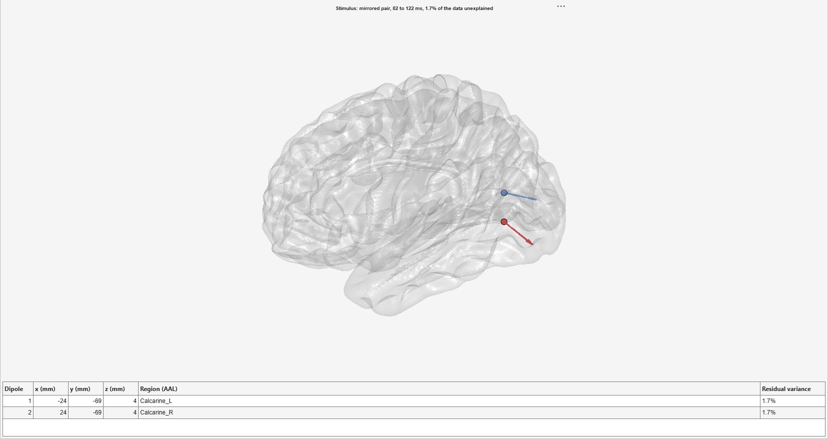
An equivalent current dipole, or a pair mirrored across the midline, fitted to a bin’s scalp distribution over a time window: where one focal generator (or one in each hemisphere) would have to be to produce it, and how much of the data it then explains. The fit is FieldTrip’s ft_dipolefitting (Oostenveld et al. 2011) on the template head model the source estimates use: a grid search over the brain for the starting point, then a nonlinear fit. The model holds the position fixed over the window and lets the moment change within it (FieldTrip’s regional model). The data are not changed; the dipoles are stored with them, and the view draws them on a see-through template brain with a table of their positions.
| Option | Default | Meaning |
|---|---|---|
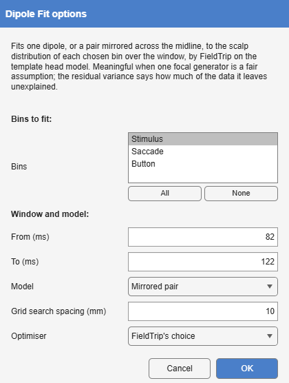
| Bins | the first | The bins to fit, each on its own. |
| From, To | 20 ms either side of the largest global field power after the event | The window, in ms. |
| Model | One dipole | One dipole, or a Mirrored pair, symmetric across the midline, for a response from both hemispheres at once. |
| Grid search spacing | 10 mm | The grid the starting point is searched on. |
| Optimiser | FieldTrip’s choice | The nonlinear fit’s optimiser: FieldTrip’s own choice, as in a FieldTrip script (fminunc where MATLAB reports the Optimization Toolbox, fminsearch otherwise), or fminsearch. |
The fit runs with FieldTrip’s own defaults, as a FieldTrip script would. On a MATLAB that reports the Optimization Toolbox without having all of it installed, FieldTrip’s choice, fminunc, stops with an error, and FieldTrip returns only the grid search’s starting point; Dipole Fit then refuses the fit and says so. Choose fminsearch there.
A dipole is the right model only when one focal generator (or one in each hemisphere) is a fair assumption, as for an early sensory response; it is not the right model for a component with distributed generators, such as the N400. The residual variance, the share of the scalp data in the window the dipoles do not reproduce, is the check, and the view puts it in the title. A low value says the model can explain the map, not that the generator is where the dipole is: with a template head and template electrode positions, a position is good to a centimetre or two. Each dipole is named by the AAL region at or within 10 mm of it, by FieldTrip’s ft_volumelookup, since a fitted dipole often lies just beneath the cortex.
The example is an early sensory response: the visual response to the faces in Ehinger and Dimigen’s recording (Overlap correction by deconvolution), in the plain average of the Stimulus bin (454 trials), around its first peak at 102 ms, strongly positive over O1 and O2. From 82 to 122 ms a mirrored pair lands in the calcarine cortex of each hemisphere, at ±24, -69, 4 mm, and leaves 1.7% of the data unexplained. A single dipole over the same window leaves only 2.4%, yet sits on the midline, in the cerebellar vermis, between the two hemispheres’ generators: the two models fit almost equally well, and only one of them is where the visual cortex is.