RESS

A plugin for Alakazam

Tools > 4. Frequency and Component Analysis > RESS · epoched, with bins → the same, with added channels · RESS

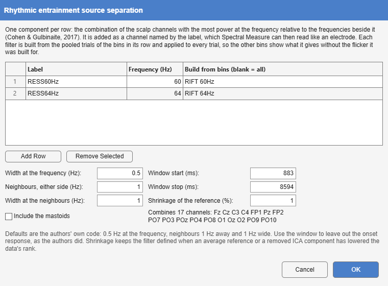
Rhythmic entrainment source separation (Cohen and Gulbinaite 2017). A tagged response is usually read from the electrode where it looks strongest, a choice that differs between people and frequencies and is circular when made on the response itself. RESS replaces it with a spatial filter per recording and frequency: the weighting of all scalp channels whose power at the stimulation frequency is largest relative to the frequencies beside it. Each filter is added as a channel (RESS60Hz), so that everything downstream, Spectral Measure’s coherence to a photodiode, SNR and ITC, reads it like an electrode.

Figure 1: RESS for the RIFT design: one row per tagged frequency, each built from its own bins, with the reference code’s filter widths.

Table 1: RESS’s options. The defaults are those of the authors’ code.

Option	Default	Meaning
rows: Label, Frequency, Build from bins		One component per row, built from the pooled trials of the listed bins (blank: all).
Width at the frequency	0.5 Hz	FWHM of the narrow Gaussian filter at the frequency.
Neighbours, either side	1 Hz	Distance of the reference frequencies.
Width at the neighbours	1 Hz	FWHM of the filters at the neighbours.
Window start, Window stop	whole epoch	The samples entering the covariances, to leave out the onset response.
Shrinkage of the reference	1%	Regularisation of the reference covariance (below).
Include the mastoids	off	Include mastoid channels among the scalp channels combined.

The method. Two channel covariance matrices are formed from the same samples: S from the data filtered narrowly at the frequency, and R as the mean of the covariances at the frequency minus and plus the neighbour distance. The generalised eigenvector of (S, R) with the largest eigenvalue maximises the ratio of power at the frequency to power beside it. The filters are Gaussians in the frequency domain, applied to the whole epoch before the window is taken. The forward model (the component’s scalp map) is $S\mathbf w / (\mathbf w^\top S \mathbf w)$, and the sign is fixed so that the largest element of the map is positive; unlike the reference code, the weights are flipped with it, so that the component’s phase, and its phase lag to a photodiode, is not arbitrary.

Shrinkage. An average reference, an interpolated channel or a removed ICA component lowers the rank of the data, and a singular R has no well-defined generalised eigenvectors. R is therefore shrunk towards a multiple of the identity, $(1-g)R + g\,\overline{\lambda}(R)\,I$; 0 reproduces the article, which used full-rank data.

Which trials. A filter built from every condition at a frequency compares those conditions fairly, because none had the filter fitted to it alone, as the authors advise. The component is then computed for every trial, so it is also applied to the bins it was not built from, and those are its null: what the filter gives where its flicker was absent. A recording without a row’s bins gets that component as all-missing, with a note, so that every recording keeps the same channels.

Only scalp EEG channels are combined, never eye channels, a photodiode or an earlier component; running RESS again replaces its channels. The weights, maps and eigenvalues are kept for the report.

Figure 2: The spectrum of the 60 Hz RESS component in the same trials: SNR at 60 Hz about 460, against about 100 at Oz (the Alakazam manual), with the 50 Hz line noise largely gone.

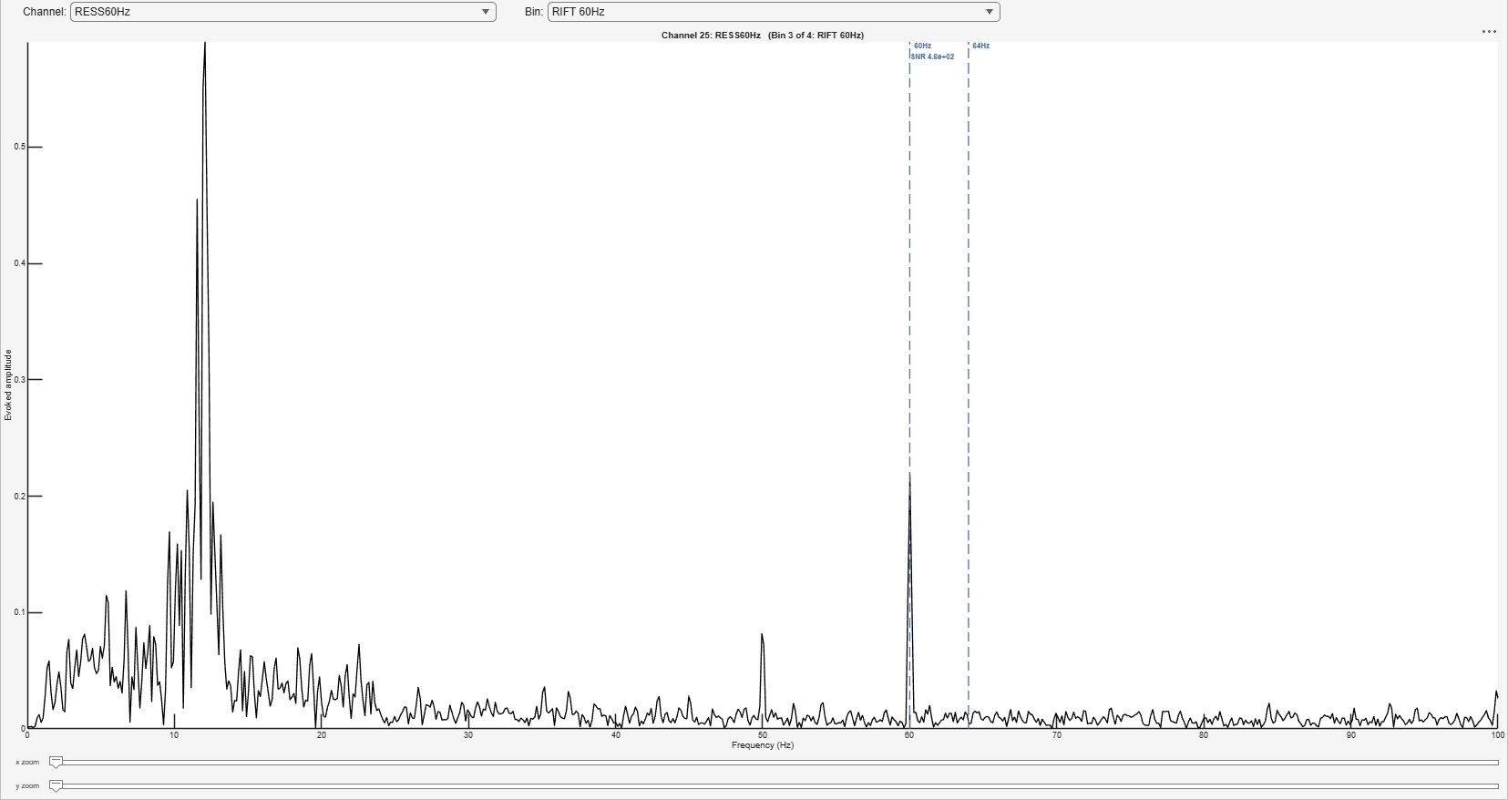
Toolbox or own code. No toolbox implements RESS. Alakazam’s follows Cohen and Gulbinaite’s own script (Cohen and Gulbinaite 2017) and reproduces its filters to ten decimals.

References

Cohen, Michael X., and Rasa Gulbinaite. 2017. ‘Rhythmic Entrainment Source Separation: Optimizing Analyses of Neural Responses to Rhythmic Sensory Stimulation’. NeuroImage 147: 43–56. https://doi.org/10.1016/j.neuroimage.2016.11.036.